Article
citation information:
Żukowska, M., Krasuski, K., Wierzbicki, D. Determining the accuracy
of a digital terrain model based on image data obtained from an unmanned aerial
vehicle. Scientific Journal of Silesian
University of Technology. Series Transport. 2025, 129, 293-309. ISSN: 0209-3324. DOI: https://doi.org/10.20858/sjsutst.2025.129.17
Marta ŻUKOWSKA[1], Kamil KRASUSKI[2], Damian WIERZBICKI[3]
DETERMINING THE
ACCURACY OF A DIGITAL TERRAIN MODEL BASED ON IMAGE DATA OBTAINED FROM AN
UNMANNED AERIAL VEHICLE
Summary. This article presents
and describes the results of research on determining the accuracy of a Digital
Terrain Model (DTM) developed based on image data obtained from an Unmanned
Aerial Vehicle (UAV). The Digital Terrain Model was created using image data acquired
by an Unmanned Aerial Vehicle, specifically the fixed-wing with electric
propulsion, flying at an altitude of 300 meters. The image data were collected
during a photogrammetric survey conducted over a mountainous area in 2021. The
final elevation values of the Digital Terrain Model were recorded in a GRID
format with a spatial resolution of 5 meters. The article also includes a
comparison of the DTM elevations with results obtained from the satellite GPS
RTK technique. Based on this, an accuracy of elevation determination for
different vertical profiles ranged from 0.19 m to 0.24 m was obtained.
Moreover, the study also involves the development of a DTM from data acquired
by the Unmanned Aerial Vehicle at an altitude of 150 meters. In this case, the
accuracy of determining the elevations of the DTM for different vertical
profiles ranged from 0.10 m to 0.16 m. The results of the research are very
interesting for the application of UAV technology in aerial photogrammetry,
particularly in inaccessible areas, especially mountainous regions.
Keywords: low altitude photogrammetry, DTM, Unmanned Aerial Vehicle,
interpolation, accuracy
1.
INTRODUCTION
Due
to the intense development of Unmanned Aerial Vehicle (UAV) technology, these
platforms are increasingly being utilized in the field of photogrammetry. Image
data obtained from UAVs enables the acquisition of a range of fundamental
photogrammetric products that find applications in numerous domains related to
spatial information. Moreover, UAVs, owing to their size, constitute an
excellent photogrammetric tool for conducting surveys over inaccessible areas
such as mountainous terrains [1]. Most such platforms are equipped with
gyroscopic stabilization and allow for autonomous flight missions.
Additionally, the costs associated with such systems and their operational
expenses are significantly lower compared to traditional methods of acquiring
aerial photogrammetric data. A significant limitation of this technology for
low-altitude image data acquisition is the use of cheap, single-frequency GPS
receivers coupled with an INS system. This results in image data being burdened
with several-meter positioning errors, which in turn affects the final accuracy
of the photogrammetric work.
One
of the potential applications of UAVs in aerial photogrammetry is the
generation of a Digital Terrain Model (DTM). A DTM is one of the primary
sources of information about the topographic surface of the terrain,
characterizing the topographic surface through a discrete network of
measurement points with known coordinates (X, Y, Z). When it also includes
information regarding the surface situation, it is referred to as a Digital
Surface Model (DSM). Therefore, a DSM represents the terrain along with its natural
(e.g., trees) or artificial (e.g., buildings) coverage [2],[3]. A DTM can be
generated based on various data sources. Appropriately processed data should
consist of information about the terrain's elevation and accurately represent
its shape. Currently, for the purposes of photogrammetric works, the main
sources of data are field measurements, aerial laser scanning, and image data
from classical aerial photogrammetry [4]. Traditional aerial photogrammetry has
long been the main and simultaneously economical source of topographic surface
elevation data. In the last decade, this role has been taken over by data
obtained through aerial laser scanning LIDAR, and the ability to develop large
areas necessitates particular attention to this method. A significant advantage
of LIDAR is that some laser pulses reflect off the terrain coverage surface,
such as forest canopies, while some (about 30% in summer and 70% in winter)
penetrate vegetation and reflect off the topographic surface, providing
information about the height of terrain coverage elements and the ability to
generate both DTM and DSM [5]. As LIDAR technology remains expensive, many
countries prefer to create photogrammetric products like DTM from images
acquired with UAVs. In recent years, small UAVs equipped with imaging sensors
offer a low-budget form of acquiring low-altitude image data, which can then be
processed into a dense point cloud using the Structure from Motion (SfM) algorithm family [6], [7]. This allows for the
generation of DTMs and DSMs and, consequently, one of the main products of
low-altitude photogrammetry – orthophotomaps.
1.1. Related
works
In
the literature, there are numerous studies on the accuracy analysis of Digital
Terrain Models (DTMs) generated based on images acquired from low altitude. In
the research conducted by Udin et al. [8], the accuracy of a DTM created from
UAV images captured with a non-metric Canon PENTAX W90 camera was examined. The
study established a photogrammetric network consisting of 23 points with known
X, Y, and Z coordinates. Sixteen of these were used as ground control points
(GCPs), and seven as independent check points (ICPs) to assess accuracy. The
analysis of the DTM accuracy was based on the Root Mean Square Error (RMSE) of
the Z-coordinate, obtaining an accuracy of less than one meter. In the work of
Akturk et al. [1], the accuracy of a DTM for areas with varied terrain was
investigated using UAV image data. The results indicated that the DTM accuracy
(RMSE value) was 0.57 m. The use of ground control points during the DTM
generation process reduced the RMSE value by 0.06 m. Uysal et al. evaluated the
DTM accuracy using 30 control points and achieved a total vertical accuracy of
0.062 m at a flying height of 60 m. The findings demonstrate that UAV
photogrammetry data can achieve suitable accuracy, very similar to RTK GPS
data, thus enabling the use of UAV photogrammetric data for creating maps,
geodetic measurements, and other engineering applications at low cost, time
savings, and minimal fieldwork. Additional studies [9] on DTM accuracy have
proven that factors such as flight planning, fieldwork, camera settings on the
UAV platform, and an adequate number of ground control points can enhance the
accuracy of the generated terrain models. In research by Jamalulizam
et al. [10], the accuracy of a DTM based on UAV data acquired at various flight
altitudes was examined, concluding that a flight altitude of 300 m provides a
more accurate terrain surface model compared to a flight altitude of 400 m.
1.2. Research
Purpose
The paper is structured as follows: in Section 2 the
research method is explained. Section 3 presents the material and experimental
results. In Section 4 the results are discussed. Finally, Section 5 provides a
brief summary of this work.
2. METHODS
The process of generating a Digital Terrain Model
(Fig. 1) based on data acquired from the UAV consists of the following steps:
data import into specialized software, image adjustment, georeferencing of
images using check points to optimize camera position and orientation, dense
point cloud generation, point cloud filtering (feature classification), DTM
generation, DSM generation and orthomosaic creation.
Fig.
1. Workflow to generate DTMs
3. MATERIALS
AND EXPERIMENTAL RESULTS
3.1. Study
area
Image
data for the research experiment was acquired using a fixed-wing system
equipped with a Sony camera. The photogrammetric raid was carried out in March
2021 under moderate photographic conditions. The test area was the vicinity of
the town (Małopolskie Voivodeship) in southern
Poland.
Ten ground control points and five check points were
used for the analyses. All points were signaled, and their coordinates were
determined using the GPS RTK technique with an accuracy of no worse than 0.05 m
(mountainous terrain). The test block consisted of 100 images acquired from an
altitude of 300 m (see Fig. 2). The aerial images were arranged in 10 strips
and the field pixel size was 0.10 m.
Image
data processing was performed in the commercial software UASMaster
[11]. After automatic digital aerotriangulation, the
mean-square error value of a typical observation was 5.1 µm (1.1 pixels). For
the check points, the mean square error values for the X, Y, and Z coordinates
were 0.10 m, 0.12 m and 0.23 m, respectively. In a further step, a dense point
cloud was generated, which was then subjected to a filtering process. The
generated Digital Terrain Model was saved as a regular GRID screen with a spatial
resolution of 5 m (see Fig. 3).
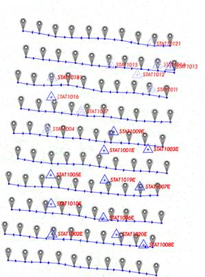
Fig.
2. The visualization of the test photogrammetric block – altitude 300 m
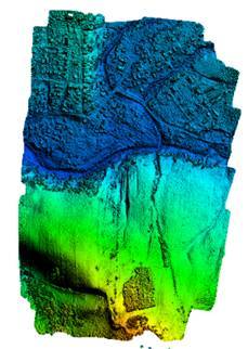
Fig.
3. The visualization of the test photogrammetric block – altitude 300 m
Tab. 1
Parameters
of the test block
|
DTM development area |
0.9 km2 |
|
Form of DTM presentation |
regular GRID |
|
Number of GRID nodes |
34666 |
|
Density of points |
4 points /
25 m2 |
|
Mesh |
5 m |
|
Average elevation |
642.40 m |
|
DTM height
range |
from 604.02 m to 732.06 m |
Table
1 shows the basic parameters of the DTM compiled from aerial imagery from the
UAV platform. The size of the DTM compilation was approximately 0.9 km2,
assuming a point density of 4 points per 25 m2. The total number of
GRID grid node points in the DTM was 34666 for a grid
mesh of 5 m. In addition, the average height of the DTM was 642.40 m, with
ground denivelations ranging from 604.02 m to 732.06 m.
3.2.
Experimental results
This
chapter presents the results of a comparison of selected DTM profiles whose
heights were determined by an interpolation model and by GPS RTK satellite
measurements. A total of three field profiles of DTM heights were analyzed. For
the interpolation model, the nearest neighbor method was used, where the
heights of the interpolated profile points were determined based on a weighted
average, as follows:
![]() (1)
(1)
where:
![]() –
interpolated height for a given profile point,
–
interpolated height for a given profile point,
![]() –
weight,
–
weight,
![]() ,
,
![]() ,
,
![]() – plane rectangular coordinates of the profile
point for which the height is being interpolated,
– plane rectangular coordinates of the profile
point for which the height is being interpolated,
![]() – rectangular planar coordinates of a
neighboring point on the regular GRID grid,
– rectangular planar coordinates of a
neighboring point on the regular GRID grid,
![]() –
serial number,
–
serial number,
![]() – number of points used to interpolate a
single height,
– number of points used to interpolate a
single height,
![]() – height of a
neighboring point from the regular GRID grid.
– height of a
neighboring point from the regular GRID grid.
The
interpolation process selects neighboring points with
coordinates ![]() , whose
distance from the interpolated point
, whose
distance from the interpolated point ![]() is less than 5 m, i.e. the mesh of the regular
GRID. The weight parameter in formula (1) is defined as a function of the
inverse distance [13] and expressed in the unit [1/m2]. The heights
of neighboring points from the regular GRID mesh are
given in meters.
is less than 5 m, i.e. the mesh of the regular
GRID. The weight parameter in formula (1) is defined as a function of the
inverse distance [13] and expressed in the unit [1/m2]. The heights
of neighboring points from the regular GRID mesh are
given in meters.
In
the second survey method, the coordinates of the selected DTM profiles were
measured using GNSS satellite technology for the GPS RTK difference method. In
the GPS RTK method, user coordinates are determined by dual-frequency phased
GPS observations at L1/L2 frequencies using a double-difference technique. In
the research test, a Leica Viva L1/L2 satellite receiver was used to measure
the pickets in the field. The typical accuracy of the terrain elevation
coordinate determination was approximately 0.05 m. The GPS RTK solution used
correction corrections from the state-owned ASG-EUPOS receiver network.
Figures
5, 6, and 7 show a diagram of the distribution of measured control points for
verification of DTM height determination. For profile no. 1, 32 pickets were
measured over an area of approximately 0.3 km2. On the other hand,
for profile no. 2, 51 pickets were measured over an area of approximately 0.005
km2. However, for profile no. 3, 39 pickets were measured over an
area of approximately 0.002 km2.
Fig. 4. The
measurement points of profile no. 1 in the testing area
Figures
7, 8 and 9 show the DTM profile height values based on the interpolation model
and the GPS RTK method. The scatter of the obtained DTM profile height results
for the interpolation model is:
-
from 608.35 m to 686.01 m for profile no. 1,
-
from 643.19 m to 651.78 m for profile no. 2,
-
from 644.27 m to 692.80 m for profile no. 3.
For
the GPS RTK method, the scatter of DTM profile height results is respectively:
-
from 608.46 m to 686.02 m for profile no. 1,
-
from 643.01 m to 651.77 m for profile no. 2,
-
from 644.20 m to 692.70 m for profile no. 3.
Fig. 5. The
measurement points of profile no. 2 in the testing area
Fig. 6. The
measurement points of profile no. 3 in the testing area
Figures
10, 11 and 12 then present the height difference of the measured DTM profile
based on the interpolation model and the GPS RTK method. The value of the
difference was determined based on the relationship:
![]() (2)
(2)
where:
![]() –
altitude from the GPS RTK measurement for a given profile point.
–
altitude from the GPS RTK measurement for a given profile point.
Fig. 7. The
elevation of profile no. 1 in the interpolation model and GPS RTK method
Fig. 8. The
elevation of profile no. 2 in the interpolation model and GPS RTK method
In
addition, for height difference dH, accuracy
parameters were determined in the form of mean absolute error ![]() and mean
squared error
and mean
squared error ![]() as recorded below:
as recorded below:
![]() (3)
(3)
and
![]() (4)
(4)
where:
![]() –
number of all measured pickets.
–
number of all measured pickets.
Fig. 9. The
elevation of profile no. 3 in the interpolation model and GPS RTK method
Fig. 10. The
elevation difference of profile no. 1 between the interpolation model
and GPS RTK method
For
profile no. 1 (Fig. 11), the average value of the dH
parameter is equal to -0.07 m, with the scatter of the dH
parameter results ranging from -0.67 m to almost 0.26 m. The error value of ![]() is equal to
0.24 m, while the parameter
is equal to
0.24 m, while the parameter ![]() is equal to
0.18 m.
is equal to
0.18 m.
On
the other hand, for profile no. 2 (Fig. 12), the average value of the dH parameter is equal to 0.12 m, with the scatter of
the dH parameter results ranging from -0.20 m to
almost 0.41 m. The error value of ![]() is equal to 0.19 m, while the
is equal to 0.19 m, while the ![]() parameter is equal to 0.16 m.
parameter is equal to 0.16 m.
In
addition, for profile no. 3 (Fig. 12), the average value of the dH parameter is equal to 0.14 m, with the scatter of
the dH parameter results ranging from -0.26 m to
approximately 0.60 m. The error value of ![]() is equal to 0.21 m, while the parameter
is equal to 0.21 m, while the parameter ![]() is equal to 0.15 m.
is equal to 0.15 m.
Fig. 11. The
elevation difference of profile no. 2 between interpolation model
and GPS RTK method
Fig. 12. The
elevation difference of profile no. 3 between the interpolation model
and GPS RTK method
4. DISCUSSION
The
discussion chapter is divided into three parts. In the first part, the trend of
change of the DTM height difference was determined in the form of a linear
regression. In the second part, the repeatability of the proposed test
methodology for the images obtained from the 150 m altitude was performed. The
third part of the discussion is a comparison of the obtained survey results in
relation to the literature on the subject.
In
the first part of the discussion, Figures 15, 16 and 17 show the nature of the
variation of the parameter dH in the form of a
1st-degree polynomial (linear regression function), which is described by the
relation [13]:
![]() (5)
(5)
where:
![]() – next picket number,
– next picket number,
![]() – linear coefficients of the 1-degree
polynomial determined.
– linear coefficients of the 1-degree
polynomial determined.
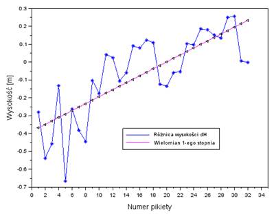
Fig. 13. The
linear regression of values of the ![]() parameter from profile no. 1
parameter from profile no. 1
Fig. 14. The
linear regression of values of the ![]() parameter from profile no. 2
parameter from profile no. 2
The
determined coefficients (a,b) from equation
(5) are obtained by applying the method of least squares taking into account
the values of dH for all measured pickets. For
profile no. 1, the nature of the changes in the parameter is positive, as evidenced by the
value of the linear parameter "a" equal to 0.019. The value of the
parameter "b" is negative and equal to -0.387 m for the measurements
adopted in the calculations. The error of fit of the linear regression function
against the actual values of dH is 0.14 m.
Furthermore, the distribution of corrections during the numerical calculations
ranged from -0.22 m to 0.38 m. Subsequently, for profile no. 2, the nature of
the changes in the parameter dH is negative
and the values of the linear coefficients are a= -0.007 and b= 0.303,
respectively. The error of fit of the linear regression function with respect
to the actual values of dH is 0.11 m and the
distribution of the corrections is described by the range of values (-0.25 ÷
0.16) m. Then, for profile no. 3, the nature of the changes in the dH parameter is positive, and the values of the linear
coefficients are a= 0.001 and b= 0.118, respectively. The error of fit of the
linear regression function with respect to the actual values of dH is 0.16 m, and the distribution of the
corrections is described by a range of values from -0.47 m to 0.39 m. The final
obtained statistical values of the 1st-degree polynomial parameters for the
individual DTM profiles are presented in Table 2.
Fig. 15. The
linear regression of values of the ![]() parameter from profile no. 3
parameter from profile no. 3
Tab. 2
The
characteristic of parameters of linear regression for all DTM profiles
|
Profile |
Linear coefficients
[m] |
Distribution of amendments
[m] |
Fitting
error of linear regression [m] |
|
No. 1 |
a= 0.019 b= -0.387 |
-0.22 ÷ 0.38 |
0.14 |
|
No. 2 |
a= -0.007 b= 0.303 |
-0.25 ÷ 0.16 |
0.11 |
|
No. 3 |
a= 0.001 b= 0.118 |
-0.47 ÷ 0.39 |
0.16 |
The
second part of the discussion was to determine the accuracy of the DTM
generated from aerial photographs acquired from an altitude of 150 m. Figures
17, 18 and 19 show the difference in DTM height from interpolation and GPS RTK
measurements for the first profile. In addition, the errors ![]() and
and ![]() were calculated.
were calculated.
Fig. 16. The
elevation difference of profile no. 1 between the interpolation model
and GPS RTK method for altitude150 m
Fig. 17. The
elevation difference of profile no. 2 between the interpolation model
and GPS RTK method for altitude150 m
Fig 18. The
elevation difference of profile no. 3 between the interpolation model
and GPS RTK method for altitude150 m
For
Profile no. 1, the scatter of results of the dH
parameter ranges from -0.31 m to about 0.58m. The error value of ![]() is equal to
0.11 m, while the parameter
is equal to
0.11 m, while the parameter ![]() is 0.16 m. Next, for profile No. 2, the
results of dH
difference were from -0.22 m to about 0.22 m, and the individual errors are
is 0.16 m. Next, for profile No. 2, the
results of dH
difference were from -0.22 m to about 0.22 m, and the individual errors are ![]() =0.09 m,
=0.09 m, ![]() =0.10 m.
Finally, for profile no. 3, the values of the dH parameter ranged from -0.41 m
to about 0.41 m, and the individual errors are
=0.10 m.
Finally, for profile no. 3, the values of the dH parameter ranged from -0.41 m
to about 0.41 m, and the individual errors are ![]() =0.12 m,
=0.12 m, ![]() =0.15 m. Table
3 shows the summary comparison of
=0.15 m. Table
3 shows the summary comparison of ![]() and
and ![]() errors obtained in the process of DTM
development for image data acquired from 150 m and 300 m altitude. Based on the
obtained results of
errors obtained in the process of DTM
development for image data acquired from 150 m and 300 m altitude. Based on the
obtained results of ![]() and
and ![]() errors, it can be said that:
errors, it can be said that:
-
the accuracy expressed by the ![]() parameter increased from 20% to 44% when using
image data at the 150 m altitude than from the 300 m altitude,
parameter increased from 20% to 44% when using
image data at the 150 m altitude than from the 300 m altitude,
-
the accuracy expressed by the ![]() parameter increased from 28% to 47% when using
image data at the 150 m altitude than from the 300 m altitude.
parameter increased from 28% to 47% when using
image data at the 150 m altitude than from the 300 m altitude.
Tab. 2
Characteristics
of the accuracy of the DTM developed from
aerial photographs acquired from 150 m and 300 m altitude
|
Profile |
Height 300 m |
Height 150 m |
|
No. 1 |
|
|
|
No. 2 |
|
|
|
No. 3 |
|
|
The
final stage of the discussion concerns the comparison of the results and the
presented research method in relation to the analysis of the state of the art.
Referring
to the results presented in the article and comparing them with other
publications concerning the accuracy of Digital Terrain Models (DTMs) obtained
using low-altitude photogrammetry, several important similarities can be
observed. When compared to studies presented in publications such as [14],
similar challenges and opportunities associated with the use of UAVs in
photogrammetry are apparent. Our study indicates the effectiveness of the
weighted average method for interpolating heights from a GRID network, which
aligns with the findings of other works [6], where the accuracy of models
obtained using this method is also emphasized in comparison to standard
geodetic techniques like RTK GPS.
In
our study, where the experiment was conducted on a sample of 51 points, an
average height difference of -0.02 m and an RMS error of 0.11 m are indicators
of good quality DTM interpolation. A similar study presented in [5] also
demonstrated that low-cost UAV photogrammetry could provide sufficient accuracy
for many applications, although it highlighted the need to consider terrain
specifics, such as vegetation or topography.
The
values of the linear coefficients (a, b) determined in our study for
different profiles show that the nature of terrain height changes can vary
depending on the specifics of the measurement location. This observation is
significant in the context of discussions on DTM creation methodology and
accuracy assessment, as different areas may require the interpolation method to
be adjusted to the data specificity.
5. CONCLUSION
The
article demonstrates the feasibility of using Unmanned Aerial Vehicle (UAV)
technology, for determining the height of a Digital Terrain Model (DTM) from
images acquired at an altitude of 300 meters. The DTM was developed as an
additional product of digital aerotriangulation for
the aerial photographs obtained. The DTM coordinates for a regular 5 m GRID
were used to determine the terrain profile height, which was also measured
using GPS RTK technique. The research experiment was conducted on a sample of 51
measured points. The terrain profile height values were interpolated from the
regular GRID using the weighted average method and compared with the solution
obtained using the GPS RTK technique. The average difference in terrain profile
height from the comparison was -0.02 m, with an RMS error of 0.11 m.
Additionally, the work describes changes in the height difference parameter of
the profile using a first-degree polynomial function, with a polynomial fitting
error relative to the determined height difference values of 0.09 m.
Future
perspectives for the development of the presented methodology for determining
the accuracy of the DTM based on UAV image data could consider several avenues.
Firstly, it would be beneficial to investigate the impact of different
atmospheric and seasonal conditions on the quality of image data and their
effect on DTM accuracy. It is possible that data acquired at different times of
the year or under various lighting conditions could influence the results of
terrain height interpolation.
Secondly,
the application of advanced image processing algorithms and machine learning
techniques could improve the automation of the DTM creation process and enhance
its precision. In particular, these techniques could assist in better
identifying and eliminating potential errors and anomalies in image data.
A
third perspective involves the use of a greater number of independent check
points (ICPs) measured with GPS RTK technique, which could improve model
calibration and increase the accuracy of interpolation. Experiments with
different GRID sizes and the application of other interpolation methods, such
as kriging or splines, may also yield valuable results.
Moreover,
future research could focus on optimizing and automating the entire measurement
and computation process to further reduce the time required to develop DTMs and
decrease the costs associated with such studies.
References
1.
Erdal
Akturk, Aykut Ozan Altunel. 2019. „Accuracy assessment of a low-cost UAV
derived digital elevation model (DEM) in a highly broken and vegetated
terrain”. Measurement 136: 382-386. ISSN: 0263-2241. DOI:
10.1016/j.measurement.2018.12.101.0.
2.
Guth P.L., A. Van Niekerk, C.H. Grohmann, J-P. Muller, L. Hawker, I.V. Florinsky, D. Gesch, H.I. Reuter, V. Herrera-Cruz, S. Riazanoff,
et al. 2021. „Digital
Elevation Models: Terminology and Definitions”. Remote Sensing 13(18): 3581. DOI: 10.3390/rs13183581.
3.
Eltner
Andreas, Lars Kaiser, Carlos Castillo, Gregory Rock, Franz Neugirg, Antonio Abellán. 2016. „Image-based surface reconstruction in
geomorphometry-Merits, limits and developments”. Earth Surf. Dyn. 4:
359-389.
4.
Kosmatin
Fras Miha, Aljoša Kerin, Matevž Mesarič, Vid Peterman, David Grigillo. 2016.
„Assessment of the Quality of Digital Terrain Model Produced from Unmanned
Aerial System Imagery International Archives of the Photogrammetry”. Remote
Sensing and Spatial Information Sciences XLI-B1: 893-899. DOI: 10.5194/isprs-archives-XLI-B1-893-2016.
5.
Jiménez-Jiménez
Sergio Iván, Wilmer Ojeda-Bustamante, Manuel David Javier Marcial-Pablo, José
Enciso. 2021. „Digital terrain models generated with low-cost UAV
photogrammetry: Methodology and accuracy”. ISPRS International Journal of
Geo-Information 10(5): 285. DOI:
10.3390/ijgi10050285.
6.
Sanz‐Ablanedo
Eduardo, John H. Chandler, Pablo Ballesteros‐Pérez, José R.
Rodríguez‐Pérez. 2020. „Reducing systematic dome errors in digital
elevation models through better UAV flight design”. Earth Surface Processes
and Landforms: 45(9): 2134-2147.
7.
Long Nicolas, Bernard Millescamps, Benjamin Guillot, Frédéric
Pouget, Xavier Bertin. 2016. „Monitoring the topography of a dynamic tidal
inlet using UAV imagery”. Remote Sensing 8(5): 387.
8.
Wan
Shamsuddin Udin, Hassan Abdal Fattah, Ahmad Aizuddin, Tahar Noorazman. 2012.
„Digital Terrain Model extraction using digital aerial imagery of Unmanned
Aerial Vehicle”. In: IEEE
8th International Colloquium on Signal Processing and its Applications: 272-275. Malacca, Malaysia. 23-25 March. DOI:
10.1109/CSPA.2012.6194732.
9.
Leal-Alves
Dione C., José Weschenfelder, Maria de Lourdes Albuquerque, et al. 2020.
„Digital elevation model generation using UAV-SfM photogrammetry techniques to
map sea-level rise scenarios at Cassino Beach”. SN Appl. Sci.
2: 2181, DOI: 10.1007/s42452-020-03936-z.
10.
Mohd Zain
Jamalulizam, Wan Mohamed Wan Mat, Norezan Nazri Nordin Mohd, Sulaiman Shahid
Ali, Ma'arof Irwan, Samad Ahmad Mohd. 2022. „DSM and DTM Extraction Accuracy
Detection Utilising UAV Imagery on Different Altitudes”. In: IEEE
13th Control and System Graduate Research Colloquium (ICSGRC). Shah Alam, Malaysia, 16-20 August. DOI:
10.1109/ICSGRC55096.2022.9845130.
11.
UAS Master Tutorial for Version 11.0 and higher. 2020.
Trimble Germany.
12.
Zhu Y.,
X. Liu, J. Zhao, Zhao, J. Zhao, X. Wang, D. Li. 2019. „Effect of DEM interpolation neighbourhood on terrain
factors”. ISPRS International Journal of Geo-Information
8(1): 30.
13.
Osada Ewa. 2001. Geodezja.
[In Polish: Geodesy]. Wrocław University of
Science and Technology Publishing House. ISBN: 83-7085-663-2.
14.
Uysal Mustafa,
Ahmet S. Toprak, Nedim Polat. 2015. „DEM generation with UAV Photogrammetry and
accuracy analysis in Sahitler hill”. Measurement 73: 539-543. ISSN: 0263-2241. DOI: 10.1016/j.measurement.2015.06.010.
Received 16.06.2025; accepted in revised form 08.09.2025
![]()
Scientific Journal of Silesian
University of Technology. Series Transport is licensed under a Creative
Commons Attribution 4.0 International License