Article
citation information:
Ta
Duc, Q., Nguyen Xuan, K., Nguyen Tuan, N., Nguyen Thanh, V., Le Dinh, M.,
Trinh Duy, H. Evaluation of SVR and random forest models for accurate prediction of
electronic fuel injector behavior in common-rail systems. Scientific Journal of Silesian University of Technology. Series
Transport. 2025, 129, 225-235. ISSN:
0209-3324. DOI: https://doi.org/10.20858/sjsutst.2025.129.13
Quyet TA DUC[1],
Khoa NGUYEN XUAN[2],
Nghia NGUYEN TUAN[3],
Vinh NGUYEN THANH[4],
Manh LE DINH[5],
Hung TRINH DUY[6]
EVALUATION OF SVR
AND RANDOM FOREST MODELS FOR ACCURATE PREDICTION OF ELECTRONIC FUEL INJECTOR
BEHAVIOR IN COMMON-RAIL SYSTEMS
Summary. In this study, machine
learning algorithms were applied to predict the main injection quantity in a
high-pressure common rail system on a diesel engine test bench. The input
parameters included engine load, fuel pressure, injection speed, and pulse
time. Two models were selected for comparison: Support Vector Regression (SVR)
and Random Forest (RF). The results showed that on the training dataset, the RF
model outperformed SVR, with RMSE and MAE values of 0.027362 and 0.017628
respectively, significantly lower than those of SVR (RMSE = 0.051563, MAE =
0.027733). Additionally, RF achieved a higher coefficient of determination
R² (0.995759 vs. 0.984939), indicating better learning of the
relationships among variables. However, on the test dataset, SVR demonstrated
superior predictive accuracy, achieving RMSE = 0.050097, MAE = 0.027673, and
R² = 0.983550, while RF showed higher RMSE (0.060355), greater MAE
(0.040485), and lower R² (0.976123). These results indicate that SVR has
better generalization capability and is less prone to overfitting than RF. To
assess the contribution of each input parameter, SHAP (SHapley
Additive exPlanations) analysis was employed. The
results revealed that injection speed, pulse duration, and fuel pressure had
the most significant impact on the injection quantity. Meanwhile, engine load
had a relatively lower influence but still played an important role under
certain operating conditions. These analyses not only provide an intuitive
understanding of model sensitivity but also help identify key factors to
prioritize in control strategies. This study lays a foundation for the
development of optimized control systems aimed at accurately and effectively
reducing engine emissions in the future.
Keywords: common rail, SVR, RF, injection speed, injection pressure
1.
INTRODUCTION
One of the most critical factors directly
influencing diesel engine performance and emissions is the fuel injection
process. In this regard, the high-pressure common rail injection system with
its advanced injector design and precise control over injection timing,
pressure, and fuel quantity, plays a pivotal role. Consequently, conducting
in-depth research on injector operation within the common rail system, is not
only vital for enhancing fuel efficiency but also represents a key approach to
minimizing harmful environmental emissions.
Federico Perini and colleagues [1] developed a
simplified phenomenological model to simulate the fuel injection rate of the
Bosch CRI2.2 injector within a common rail system. This model enables accurate
predictions of the injection process without requiring detailed structural data
of the injector. After being calibrated with experimental data, the model is
used as an input for computational fluid dynamics (CFD) simulations in engines.
The results demonstrate the model's capability to precisely predict injection
rates and equivalence ratio distributions while maintaining reliability across
various fuel flow rates and injection pressures. Tantan Zhang [2] introduced a
real-time method for evaluating large fuel injection quantities (greater than 6
mg per injection) in common rail systems by integrating an additional pressure
sensor into the fuel pipe. The pressure data obtained from the sensor is analyzed using an artificial neural network (ANN) combined
with a physical model to accurately estimate the injected fuel mass. This
approach achieves an error margin of just 1.4 mg, indicating strong potential
for practical applications in fuel injection monitoring and precise control.
Jianhui Zhao and colleagues [3] developed a deep learning model based on a
General Regression Neural Network (GRNN) to accurately predict the fuel
injection quantity in common rail systems. To enhance model performance, the
research team applied the Particle Swarm Optimization (PSO) algorithm to
fine-tune network parameters, thereby improving prediction accuracy. The
results showed an average error of only 1.10%, with a coefficient of
determination (R²) reaching 0.997. Tests conducted under 144 different
operating conditions further revealed a maximum deviation reduction of up to
62.02% in the main injection quantity, highlighting the model's outstanding
capability in accurately controlling multiple injection cycles. Synthesizing
the above studies, it is evident that machine learning methods have become
increasingly prevalent and widely applied in forecasting and identifying the
optimal operating regions of injectors and engines [4 -7]. While many previous
studies have focused on simulating and predicting injector behavior
in common rail systems, most have relied primarily on CFD simulations or
employed a single machine learning model. Although CFD offers high accuracy, it
often involves high computational costs and long processing times, which limits
its practicality in real-time applications. On the other hand, studies using
machine learning often implement only one algorithm, lacking comprehensive
comparisons and evaluations among different methods. Based on this context, the present study
proposes and compares two widely used machine learning models Support Vector
Regression (SVR) and Random Forest (RF) for predicting the behavior
of electronic fuel injectors. Evaluating the performance of these models not
only facilitates the selection of the most suitable algorithm for a specific
application but also offers a more comprehensive perspective on the potential
of machine learning in analyzing and optimizing fuel
injection systems. This constitutes the novelty and key contribution of the
study compared to previous works.
2. METHODOLOGY
Support Vector
Regressor (SVR)
SVR
aims to find a regression function of the form:
f(x) = ωT φ(x) + b (1)
Where: ω is the weight
vector, ϕ(x)
is the feature mapping function that transforms the input data 𝑥 into a
higher-dimensional feature space, and 𝑏 is
the bias term.
Random Forest
(RF)
Random
Forest (RF) is an ensemble machine learning algorithm that combines the outputs
of multiple individual models to generate a single, more accurate prediction.
In this study, the RF model is built upon decision trees, where each tree
independently splits nodes and makes predictions. RF employs the bagging
technique, in which each decision tree is trained on a randomly sampled subset
of the original dataset, allowing for model diversity and improved
generalization. In regression tasks, the final prediction is computed by
averaging the outputs of all individual trees. By aggregating the results from
multiple base learners, the RF model enhances prediction accuracy and
effectively reduces the risk of overfitting [8]. Given the dataset’s
significant feature imbalance, an 80:20 train-test split is applied. Techniques
such as cross-validation, learning curves, and residual analysis are utilized
for model evaluation. This study employs a pipeline model with GridSearchCV to systematically experiment with both linear
and nonlinear regression models, covering the entire process from data
preprocessing to model training. The dataset is normalized using the Standard
Scaler method [9]. The goal of the predictive model is to identify a function
that minimizes the difference between predicted and actual values. This
difference is quantified by a loss function, and the machine learning model
aims to optimize this loss function. The following section presents common
error metrics used for model evaluation [10].
Mean
Squared Error (MSE) Calculates the mean square of the model error:
![]() (2)
(2)
Root
Mean Squared Error (RMSE) calculates the average deviation between predicted
values and actual values.
![]() (3)
(3)
Mean
Absolute Error (MAE) calculates the average of the absolute errors between the
actual and predicted values.
![]() (4)
(4)
R²
(Coefficient of Determination): A statistical indicator that shows the
proportion of variance in the target to be predicted that is explained by the
input variables in the model.
![]() (5)
(5)
Mean
Absolute Percentage Error (MAPE).
![]() x 100 (6)
x 100 (6)
Where: yi is the actual value and ![]() is
predicted value,
is
predicted value, ![]() is
the average of the actual values.
is
the average of the actual values.
Shapley
Additive Explanations (SHAP) interpret a feature by quantifying its
contribution to the model’s prediction. The SHAP value of a feature represents
how much that feature adds to or subtracts from the model's output compared to
the average prediction. When the input value of a feature changes, its
corresponding SHAP value also changes, reflecting the variation in that
feature’s influence on the model’s prediction. This change can be linear or
nonlinear, depending on the nature of the model and interactions with other
features [11]. The use of standard deviation and mean error [12], calculated
through Equations (7), (8) and (9).
![]() (7)
(7)
![]() (8)
(8)
![]() (9)
(9)
Where: St:
represents the standard deviation; t ̂: denotes the sample mean; t_i: is the mean error value of the individual parameter;
n: refers to the sample size.
3. RESULTS AND
DISCUSSION
Table
1 presents the fuel Table 1 presents the fuel flow rate prediction performance
of two machine learning methods Support Vector Regression (SVR) and Random
Forest (RF) using evaluation metrics including RMSE, MAE, R², and standard
deviation (STD), measured on both the training and testing datasets. On the
training set, the RF model demonstrates superior performance, achieving lower
RMSE and MAE values of 0.027362 and 0.017628, respectively, compared to SVR’s
RMSE = 0.051563 and MAE = 0.027733. In addition, RF obtains a higher
coefficient of determination (R² = 0.995759) than SVR (R² =
0.984939), indicating that RF learns the relationship between variables more
effectively during training. However, on the testing set, SVR yields more
accurate predictions, with RMSE = 0.050097, MAE = 0.027673, and R² =
0.983550, while RF results in higher error values (RMSE = 0.060355, MAE =
0.040485) and a lower R² of 0.976123. These results suggest that SVR
generalizes better and is less prone to overfitting compared to RF. Regarding
standard deviation, both models show similar levels of output variability on
both training and testing sets, indicating the stability of both the data and
the models. RF is better suited for scenarios where high accuracy on training
data is essential, whereas SVR is a more appropriate choice when prioritizing
model stability and generalizability to new, unseen data.
Tab. 1
Prediction
Results of the Models
|
Method |
Phase |
RMSE |
MAE |
R2 |
STD |
|
SVR |
Train |
0.051563 |
0.027733 |
0.984939 |
0.412498 |
|
Test |
0.050097 |
0.027673 |
0.983550 |
0.396126 |
|
|
RF |
Train |
0.027362 |
0.017628 |
0.995759 |
0.412343 |
|
Test |
0.060355 |
0.040485 |
0.976123 |
0.380328 |
Figures
1 and 2 illustrate the learning curves of two different algorithms: RSV and RF,
demonstrating how each model's performance evolves with increasing training
sample size. For the RSV algorithm, both the training score (red curve) and the
cross-validation score (green curve) show a rapid decline in error as the
number of training samples increases. Specifically, the Mean Squared Error
(MSE) of the training score starts at around 0.3 with a small dataset and
quickly drops below 0.002 when the sample size reaches approximately 50,
eventually stabilizing at around 0.001. Similarly, the cross-validation score
decreases sharply from over 0.3 to below 0.003 once the training sample size
exceeds 100. The gap between the training and cross-validation curves remains
very narrow (less than 0.002), indicating that the model learns well and
generalizes effectively, with no signs of overfitting or underfitting.
Moreover, the shaded region around the cross-validation score curve is narrow
(±0.001), suggesting high model stability across different validation sets.
These characteristics confirm that the RSV model not only fits the training
data well but also performs reliably on unseen data, making it a robust choice
for regression tasks in this context.
In
contrast, for the Random Forest (RF) algorithm, although the training score
achieves a very low MSE (below 0.005) even with a small number of training
samples, the cross-validation score remains significantly higher and decreases
only gradually as the sample size increases. Specifically, the MSE of the
cross-validation starts around 0.22–0.25 and only drops to approximately 0.01
when the number of training samples reaches 300. The gap between the training
and validation scores ranges from 0.01 to 0.02, indicating a tendency toward
overfitting; the model fits the training data very well but performs less
effectively on unseen data. Additionally, the shaded area around the
cross-validation score curve in the RF plot is noticeably wider (up to ±0.01),
reflecting a higher variance in performance across different validation sets
and hence reduced model stability.
Nevertheless,
the steady downward trend of the cross-validation score with increasing
training data suggests that RF has potential for improvement, particularly if
more training data is provided or appropriate hyperparameter tuning is
performed. This highlights the possibility of enhancing both the accuracy and
stability of the model for practical applications.
Based on the
above results, it can be concluded that the RSV algorithm demonstrates superior
performance on the current dataset, with lower MSE and fast convergence between
training and validation scores indicating strong generalization capability. In
contrast, while Random Forest (RF) shows promising potential, it currently
suffers from overfitting and requires either more training data or further
hyperparameter tuning to achieve the same level of stability and effectiveness
as RSV.
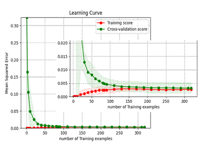
Fig.
1. Learning curve of SVR model
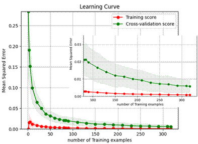
Fig.
2. Learning curve of RF model
Figure
3 illustrates a comparison between the actual values (denoted by red stars) and
the predicted results from two regression algorithms: SVR (Support Vector
Regression – represented by blue triangles) and RF (Random Forest – represented
by yellow squares) across 91 data samples in the test set. It can be observed
that both algorithms tend to produce predictions closely aligned with the
actual values. However, noticeable deviations still occur, particularly in
samples with abnormally high or low "Flow" values, such as samples
19, 34, 55, and 61. These outliers highlight specific cases where the models
struggle to maintain accuracy, especially under extreme conditions. In most
data points, both SVR and RF yield predictions that are close to the actual values;
however, differences between the two models can be observed in terms of
fluctuation and adherence to the true data trend. Specifically, SVR tends to
produce smoother and more continuous predictions, particularly in regions with
gradual variations, thanks to its ability to flexibly adapt within the function
space. In contrast, while RF is powerful in handling nonlinear relationships,
it sometimes generates abrupt or repetitive outputs due to the nature of
decision trees, leading to larger errors at boundary or transition points.
Overall, SVR demonstrates slightly higher stability and accuracy, especially in
areas with minor fluctuations in flow values. Meanwhile, RF may perform well at
certain extreme points but shows less consistency across transitional segments.
This observation aligns with the earlier Learning Curve analysis, where SVR
exhibited balanced performance between training and validation sets, while RF
showed signs of overfitting. Therefore, SVR may be the more suitable choice in
regression problems that demand high accuracy and stability on the test
dataset.
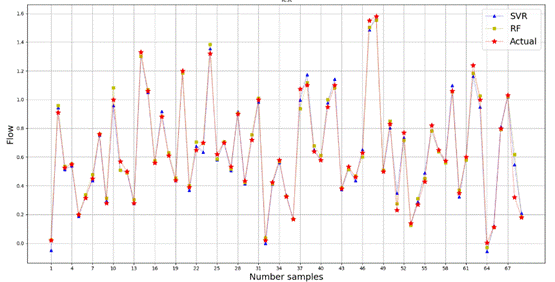
Fig.
3. Comparation prediction values on testing data between models
Figure
4 presents a comparison of the prediction performance between two machine
learning models Support Vector Regressor (SVR) and Random Forest (RF) in a
regression task. The left plot shows the results for SVR, while the right plot
displays those for RF. Both plots illustrate the relationship between the
actual values (y-axis) and the predicted values (x-axis), with the red dashed
line representing the ideal prediction line, where predicted values perfectly
match the actual values (i.e., y = x). The SVR model demonstrates highly
promising results, with a coefficient of determination of R² = 0.984,
indicating that the model explains 98.4% of the variance in the test data. In
addition, its error metrics are very low, with an RMSE of 0.050 and an MAE of
0.028, reflecting high prediction accuracy and model stability. Meanwhile, the
Random Forest model also performs well, achieving an R² of 0.977, RMSE of
0.060, and MAE of 0.039. Although these metrics are slightly less favorable than those of SVR, RF still delivers effective
predictions, as evidenced by the data points being closely clustered around the
y = x line. From these results, it is clear that both models perform well, but
SVR achieves slightly higher accuracy with lower prediction errors, making it better
suited to the characteristics of this particular dataset. However, the final
choice of model should also consider other factors such as training time,
scalability with larger datasets, and interpretability requirements depending
on the specific application context.
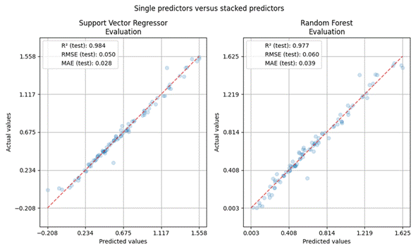
Fig. 4. Prediction results of the models on the
testing data
Figure
5 illustrates the contribution of input features to the prediction outcomes of
the Support Vector Regressor (SVR) model. Among these, Injection_speed
has the most significant impact, as evidenced by high values (in red) greatly
increasing the predicted output, while low values (in blue) tend to decrease
it. The next two influential features, Pressure and Pulse_time,
also demonstrate substantial effects pressure typically contributes to higher
predictions when its value is high, whereas Pulse_time
exhibits both positive and negative influences, indicating a more complex
relationship with the output. In contrast, the features related to speed at
different channels (Speed_CH_1: Low-speed mode, representing light load and low
engine speed conditions; Speed_CH_2: Medium-speed mode, reflecting typical
operating conditions in real-world usage; Speed_CH_3: High-speed mode,
corresponding to situations where the engine operates at high power or under
heavy load; and Speed_CH_4: Medium-speed mode combined with a pilot injection
strategy) show noticeably smaller impacts, with SHAP values mostly close to
zero. Overall, this plot reveals that the SVR model primarily relies on the top
three features for making predictions. This insight is crucial for model
interpretability, feature selection, and improving forecasting performance.
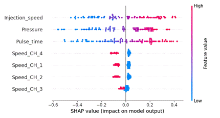
Fig. 5. SHAP
value chart
Figure
6 illustrates the mean absolute SHAP values (mean (|SHAP value|)) for each
feature, reflecting the average impact of each feature on the output of the SVR
model. Among them, the three most important features are Injection_speed,
Pressure, and Pulse_time, with mean SHAP values of
approximately 0.205, 0.200, and 0.195, respectively. These values indicate that
they contribute the most to adjusting the model's prediction results. In
contrast, the features related to load conditions represented by low load,
medium load, high load, and pilot injection are shown through the corresponding
input variables (Speed_CH4, Speed_CH1, Speed_CH2, and Speed_CH3), which exhibit
significantly lower average SHAP values of about 0.045, 0.040, 0.038, and
0.025, respectively. This indicates that the speed features in these channels
have a relatively minor influence on the model. The inclusion of these
quantitative values helps clarify the relative importance of the features,
effectively supporting feature selection and dimensionality reduction. As a
result, the model can be simplified, leading to improved processing
performance.
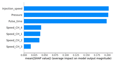
Fig. 6. The
influence of input features on the model output
4. CONCLUSION
In
this study, two machine learning models Support Vector Regression (SVR) and
Random Forest (RF) were developed to predict fuel injection quantity and assess
the influence of input parameters such as injection speed, pressure, pulse
duration, and operating modes on the injector performance in the diesel
engine's common rail system. The results show that both models achieved high
predictive performance. In particular, the SVR model demonstrated superior
accuracy, with a coefficient of determination 𝑅² = 0.984, explaining 98.4%
of the variance in the test dataset. Low error metrics, including RMSE = 0.050
and MAE = 0.028, further confirm the model’s stable and accurate predictive
capability. The Random Forest model also delivered promising results, with 𝑅² =
0.977, RMSE = 0.060, and MAE = 0.039. Additionally, the SVR model achieved an
RMSE of 5.86 MPa in terms of pressure units, indicating better generalization
across various operating conditions. The analysis of feature importance in the
SVR model revealed that the three most influential factors are injection speed,
fuel pressure, and pulse time. Among these, injection speed plays the most
critical role, followed by pressure and pulse duration, highlighting the
significance of these parameters in controlling the fuel injection system.
These findings not only clarify the role of each technical parameter in
injector control but also provide valuable support for calibration and
optimization of engine performance. Overall, this study demonstrates the
effectiveness of machine learning models in accurately predicting key technical
parameters and opens up new directions for developing intelligent control
systems aimed at enhancing engine performance and reducing emissions in diesel
engines. In the future, integrating real-time sensor data with deep learning
techniques is expected to further improve the accuracy and adaptability of
modern control systems.
Acknowledgement
This
research was funded by Hanoi University of Industry under Project
09-2025-RD/HĐ-ĐHCN
References
1.
Baker P., P.
Croucher, F. Perini, S. Busch, R.D. Reitz. 2020. „A phenomenological rate of injection model for predicting
fuel injection with application to mixture formation in light-duty diesel
engines”. Proceedings of the Institution of Mechanical
Engineers, Part D 234(7): 1826-1839. DOI: 10.1177/0954407019-898062.
2.
Tantan
Zhang. 2022. „An estimation method of the fuel mass injected in large
injections in Common-Rail diesel engines based on system identification using
artificial neural network”. Fuel
310 (Part B): 122404. ISSN:
0016-2361. DOI: 10.1016/j.fuel.2021.122404.
3.
Xiangdong
Lu, Jianhui Zhao, Vladimir Markov, Tianyu Wu. 2024. „Study on precise fuel injection under multiple injections
of high pressure common rail system based on deep learning”. Energy 307: 132784. ISSN: 0360-5442. DOI: 10.1016/j.energy.2024.132784.
4.
Yosri M., R. Palulli, M. Talei, et
al. 2023. “Numerical investigation of a large bore, direct
injection, spark ignition, hydrogen-fuelled engine”. International Journal Of Hydrogen Energy 48(46):
17689-17702.
5.
Finesso Roberto,
Ezio Spessa. 2015. “A control-oriented approach to estimate the injected fuel
mass on the basis of the measured in-cylinder pressure in multiple injection
diesel engines”. Energy Conversion and Management 105: 54-70. ISSN: 0196-8904. DOI: 10.1016/j.enconman.2015.07.053.
6.
Mengzhao
Chang, Minuk Jeong, Sungwook Park, Hyung Ik Kim, Jeong Hwan Park, Suhan Park. 2023. „Study on
predictions of spray target position of gasoline direct injection injectors
with multi-hole using physical model and machine learning”. Fuel
Processing Technology 247: 107774. ISSN: 0378-3820. DOI: 10.1016/j.fuproc.2023.107774.
7.
Junjian
Tian, Yu Liu, Haobo Bi, Fengyu Li, Lin Bao, Kai Han, Wenliang Zhou, Zhanshi Ni, Qizhao Lin. 2022. „Experimental study on the spray characteristics of
octanol diesel and prediction of spray tip penetration by ANN model”. Energy 239 (Part A): 121920. ISSN:
0360-5442. DOI: 10.1016/j.energy.2021.121920.
8.
Breiman
L. 2001. „Random Forests”. Machine
Learning 45: 5-32. DOI: 10.1-023/A:1010933404324.
9.
Manjurul
Ahsan Md, M.A. Mahmud, Pritom Saha, Kishor Datta Gupta, Zahed
Siddique. 2021. “Effect of Data Scaling Methods on Machine Learning
Algorithms and Model Performance”. Technologies
9: 52.
10.
Yingjie
Tian, Duo Su, Stanislao Lauria, Xiaohui Liu. 2022. “Recent advances on loss functions in deep learning for
computer vision”. Neurocomputing 497: 129-158. ISSN: 0925-2312. DOI: 10.1016/j.neucom.2022.04.127.
11.
Hilloulin Benoît, Van Quan Tran. 2022. “Using machine learning techniques for predicting
autogenous shrinkage of concrete incorporating superabsorbent polymers and
supplementary cementitious materials”. Journal
of Building Engineering 49: 104086. ISSN: 2352-7102. DOI: 10.1016/j.jobe.2022.104086.
12.
Kumar Shashikant,
Rakesh Kumar, Baboo Rai, Pijush Samui. 2024. “Prediction of compressive strength of high-volume fly ash
self-compacting concrete with silica fume using machine learning techniques”. Construction and Building Materials 438: 136933. ISSN: 0950-0618. DOI: 10.1016/j.conbuildmat.2024.136933.
Received 11.07.2025; accepted in revised form 04.10.2025
![]()
Scientific Journal of Silesian
University of Technology. Series Transport is licensed under a Creative
Commons Attribution 4.0 International License