Article
citation information:
Rudzinskyi, V., Lomakin, V., Melnychuk, S., Yemets, B., Lyashuk, O., Ryabchuk, O., Slobodian, L. Chaotic behavior in the rotational
speed of internal combustion engines. Scientific
Journal of Silesian University of Technology. Series Transport. 2025, 127, 237-255. ISSN: 0209-3324. DOI: https://doi.org/10.20858/sjsutst.2025.127.14
Volodymyr RUDZINSKYI[1], Volodymyr LOMAKIN[2], Serhii MELNYCHUK[3], Bogdan YEMETS[4], Oleg LYASHUK[5], Oleksandr RYABCHUK[6], Liubomyr SLOBODIAN[7]
CHAOTIC BEHAVIOR
IN THE ROTATIONAL SPEED OF INTERNAL COMBUSTION ENGINES
Summary. This study investigates
the chaotic behavior in the rotational speed of
internal combustion engines. High-precision measurements of engine rotational
speed were taken at discrete intervals of 0.36 degrees with time measured to a
precision of 41 nanoseconds. The data was analyzed
using various techniques from chaos theory and nonlinear dynamics, including
Lyapunov exponent calculations, phase space reconstruction, and power spectral
density analysis. Results reveal that engine rotational speed exhibits complex,
chaotic behavior across different operating
conditions. Lyapunov exponents ranged from -0.004 to 0.024, indicating varying
degrees of chaos from near-stability to strong chaotic behavior.
The strongest chaos was observed at certain idle speeds, while full gas
conditions showed milder but persistent chaotic characteristics. The study
demonstrates that rotational speed fluctuations in internal combustion engines
go beyond simple periodic or random variations, suggesting that traditional
linear models may be insufficient for accurately predicting and controlling
engine behavior. These findings have significant
implications for engine design, control strategies, and diagnostics. The
authors provide access to the original datasets and analysis code, encouraging
further research and collaboration in this field. This work contributes to a
deeper understanding of engine dynamics and may lead to the development of more
sophisticated, nonlinear approaches to engine analysis and optimization.
Keywords: rotational speed, rotation per minute, chaos, chaotic distribution,
internal combustion engine
1. INTRODUCTION
Chaos
theory examines the intricate behavior of nonlinear
dynamical systems, composed of interacting elements that collectively exhibit
complex behavior. These systems are termed
"nonlinear" because their interactions produce outcomes influenced by
feedback and multiplicative effects, resulting in a whole greater than the sum
of its parts. "Dynamical" indicates these systems evolve over time,
with changes depending on their current state. Many real-world systems are
nonlinear and dynamical in nature. Chaotic systems, a subset of these, can
display complex and unpredictable behavior even with
a small number of interacting components governed by simple rules. A defining
feature of chaotic systems is their sensitivity to initial conditions, where
minor differences at the start can lead to dramatically different outcomes over
time. Contrary to expectations that simple deterministic systems would yield
predictable behavior, chaotic systems can produce
highly erratic and divergent patterns. These patterns often exhibit fractal
characteristics, showing intricate and self-similar structures that never
exactly repeat. The inherent sensitivity of chaotic systems means that
long-term predictions are extremely difficult, as even the slightest
measurement inaccuracies can result in vastly different future states. Chaos
theory highlights the fundamental limits of predictability in certain systems
and suggests that precise knowledge of future states is often unattainable.
Furthermore, small interventions in chaotic systems can lead to unpredictable
consequences, as tiny changes can be amplified or diminished in complex,
nonlinear ways [1, 2].
Chaotic
processes are prevalent, and chaos theory aids in predicting behavior across various fields. Unfortunately, such a
background is not commonly applied in engineering practice. Internal combustion
engines consist of numerous small, independent processes that can exhibit
chaotic behavior. Nevertheless, the application of
chaos theory to fundamental output data such as rotational speed or power is
not widespread, though similar approaches exist in the literature, for example
[2-6]. This study aims to demonstrate a chaotic approach for better
understanding the behavior of the rotational speed of
a four-cylinder gasoline engine and ways to predict its behavior
in engineering tasks.
Previously,
the authors have studied the rotational speed and torque of internal combustion
engines for measurement parameters, diagnostics, and improving engine design.
This data allowed for the discovery of chaotic behavior
in rotational speed. The objective of experimentally tracking the rotational
speed was to achieve high resolution and accuracy in time measurement, thereby
minimizing rounding and other errors. The data collected were measured with
exceptional precision: the rotational speed was recorded at discrete intervals
of 0.36 degrees, and time was measured with a precision of 41 nanoseconds. The
authors anticipated a random distribution of rotational speed data; however,
some graphs revealed unexpected deterministic zones that resembled deterministic
chaotic series. Consequently, the goal is to investigate the chaotic nature of
the crankshaft speed distribution in internal combustion engines.
2. MATERIALS
AND METHODS
Chaos can
manifest itself in both continuous (i.e., with dynamics defined by differential
equations) and discrete (i.e., with dynamics defined by an iterated map)
nonlinear dynamical systems. One of the simplest examples is the logistic map,
a one-dimensional, discrete equation that produces chaos at certain growth
rates [1]. However, the authors aim to identify a model from experimental data
and prove chaotic behavior.
Experimental
data were collected from a ZAZ-1103 "Slavuta"
vehicle with a MEMZ-2457 motor. To ensure correct measurements, an encoder
(HEDS-9040 module and the HEDS-6140#B13 code wheel, Table 1) from AVAGO
Technologies with extra high resolution was used (1000 imp/rotation). Normally,
encoders within 100 impulses per rotation (sometimes up to 300) are used to
track rotational speed and crankshaft position. To ensure sufficient accuracy
in measuring time intervals, a quartz resonator of 24.576 MHz was used, which
provided a maximum error value of 0.38% at a motor rotation frequency of 5600
rpm [7].
Tab. 1
Characteristics of the HEDS-9040
module
and the code wheel HEDS-6140#B13 from AVAGO Technologies
|
Parameter |
HEDS-9040 |
HEDS-6140#B13 |
|
Operating
temperature range |
-40°C
to +100°C |
-40°C
to +100°C |
|
Resolution |
- |
1000
imp/rev |
|
Number
of channels |
3 |
3 |
|
Maximum
rotation frequency |
- |
30,000
rpm |
|
Permissible
shaft axial play |
±0.25
mm |
±0.25
mm |
|
Permissible
eccentricity with radial play not more than |
0.1 mm |
±0.1 mm |
|
Maximum
angular acceleration |
250,000
rad/s^2 |
250,000
rad/s^2 |
|
Maximum
error per one cycle of a discrete (%) per revolution |
5.5° |
7.5° |
|
(1.5 x
10^-3%) |
(2.1 x
10^-3%) |
|
|
Maximum
shaft position error per revolution |
40'
(0.19%) |
20'
(0.09%) |
Experiments
were conducted on the road with idle regimes at different rotational speeds and
with a fully loaded engine moving up a slope. The sensor was located closest to
the 4th cylinder, so to avoid the influence of angular oscillations of the
crankshaft, differences in sparking, fuel mixing, compression ratios in
different cylinders, etc., we tracked cycle-to-cycle series of operation for
only the 4th cylinder during only power stroke (180 deg)
[8].
In order
to analyze the chaotic behavior
of the rotational speed of internal combustion engines, a comprehensive
approach involving both qualitative and quantitative methods is necessary. The
following sections describe the data analysis model employed in this study,
incorporating various mathematical techniques and chaos theory principles.
2.1 Data
Preprocessing
The first
step in the data analysis process is to preprocess the collected experimental
data. This involves:
· Filtering and Smoothing: Noise in
the data is reduced using digital filtering techniques, such as the Savitzky-Golay filter, which smoothens the data while
preserving essential features like peak values and overall trends.
· Normalization: The data
is normalized to remove any biases due to variations in the measurement units
or scales.
· Time Series Construction: The
rotational speed data is converted into a time series format, where each data
point represents the engine's speed at a specific time interval.
2.2 Phase Space Reconstruction
Phase
space reconstruction is a crucial step in understanding the dynamics of a
chaotic system. Takens' theorem provides a framework
for reconstructing the phase space from a single time series [9]. The process
involves the following steps:
· Delay Embedding: Create a
delay coordinate matrix from the time series data. The delay embedding method
constructs vectors from the time series x(t) as follows:
x(t)=[x(t),x(t+τ),x(t+2τ),…,x(t+(m−1)τ)] (1)
where τ is the time delay
and m is the embedding dimension.
· Selection of Parameters: The
optimal time delay τ and embedding dimension m are determined using
methods like the Average Mutual Information (AMI) for τ and the False
Nearest Neighbors (FNN) algorithm for m [10].
2.3 Nonlinear Time
Series Analysis
Once the
phase space is reconstructed, various nonlinear time series analysis techniques
are applied to quantify the chaotic behavior:
·
Lyapunov
Exponents: These exponents measure the average rate of separation
of infinitesimally close trajectories in the phase space. A positive largest
Lyapunov exponent is a strong indicator of chaos. The exponents are calculated
using algorithms such as the Wolf algorithm or the Rosenstein method [11].
·
Correlation
Dimension: The correlation dimension D2 provides a measure of the
fractal geometry of the attractor. It is calculated using the Grassberger-Procaccia algorithm, which involves estimating
the scaling behavior of the correlation sum C(r) as a
function of the radius r [12]: C(r)∝rD2
·
Poincaré Sections: A Poincaré
section is a lower-dimensional representation of the system's dynamics. By
examining the intersections of trajectories with a chosen plane, one can
visualize the structure of the attractor and detect chaotic behavior.
2.4 Statistical
Analysis
In
addition to nonlinear analysis, statistical methods are used to further
characterize the rotational speed data:
·
Probability
Density Functions (PDFs): The PDFs of the rotational speed are
computed to understand the distribution and identify any anomalies or
deterministic zones.
·
Autocorrelation
Functions: The autocorrelation function R(τ) measures the
correlation between the time series and its lagged version. A rapidly decaying
autocorrelation function suggests chaotic behavior
[10].
·
Power
Spectral Density (PSD): The PSD analysis helps identify dominant
frequencies and the presence of broad-spectrum noise, indicative of chaotic
dynamics.
2.5 Surrogate Data
Testing
To
validate the presence of chaos, surrogate data testing is employed. This
involves generating surrogate data sets that preserve some properties of the
original data (e.g., amplitude distribution) but are otherwise random.
Statistical tests compare the original data with the surrogates to determine if
the observed features are genuinely due to chaos or random processes [13].
3. DISCUSSION OF THE
RESULTS OF THE EXPERIMENT
We started
to analyze data for idle mode with minimal stable
rotational speed. Data analysis done by Python with graphic user interface,
mathematical/statistical libraries and large language models (numpy, pandas, scipy, matplotlib,
sklearn ) [13-19]. Data analysis was split into 2
part to increase stability and speed of calculations. All datasets and codes
will be able to be downloaded by link [14].
The nature
of the rotation of internal combustion engine data is periodic, so
normalization should include this. It is because we track “power stroke” of the
4th engine's cylinder and skip for next 540 deg
of the crankshaft rotational for the 4th cylinder [8]. By nature of
combustion, rotational speed changing impulsivity, so normalized graph like
from mean value don’t give clear visualization of chaotic
distribution due to periodic functionality changing rotational speed with big
enough amplitude.
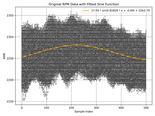
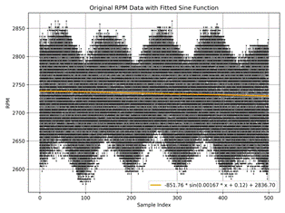
So, to clearly see the
chaotic distribution of rotational speed,
the normalization of the graph
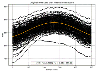
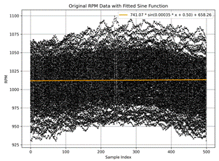
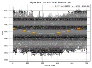
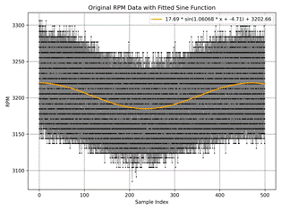
thru periodic function a·sin(b·x-c)+d (Figure 1 a)-f)) should
be made.
The graphs
a)-d) shows idle with a) ≈ 550 rpm,
b) ≈ 1010 rpm,
c) ≈2160 rpm,
d) ≈ 3200 rpm
rotational speed accordingly. The graphs e), f) show full gas regime during
moving up in the slope 12% and 10% incline, respectively.
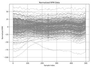
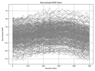
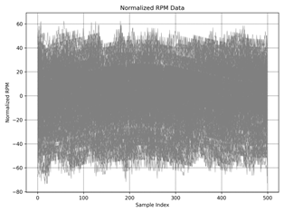
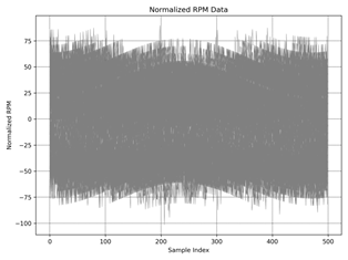
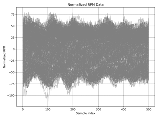
Normalized RPM data
plot for the same regimes shown in the figure
2 a)-f). Normalization scales
the data to have a mean
of a·sin(b·x-c)+d function, making it easier
to compare and analyze.
|
|
|
|
|
|
|
|
|
|
Fig. 1. Rotational Speed Data (Revolutions Per Minute) RPM with
approximation at different modes: idle a) ≈
550 rpm, b) ≈ 1010 rpm, c) ≈2160 rpm, d) ≈
3200 rpm, full gas slope 12%, |
|
|
a) |
b) |
|
c) |
d) |
|
e) |
f) |
|
Fig. 2. The normalized RPM data over the sample index: idle a) ≈ 550 rpm, b) ≈ 1010 rpm, |
|
|
a) |
b) |
|
c) |
d) |
|
e) |
f) |
|
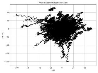
Fig. 3. Phase Space Reconstruction: idle a) ≈
550 rpm, b) ≈ 1010 rpm, c) ≈2160 rpm, |
|
|
a) |
b) |
|
c) |
d) |
|
e) |
f) |
|
Fig. 4. Average Mutual Information (AMI): idle a) ≈ 550 rpm, b) ≈ 1010 rpm, c) ≈2160 rpm, |
|
Figures 1 and 2 present
the rotational speed data and the normalized RPM, respectively. The raw data exhibits substantial variability, making it challenging to discern clear
trends. Normalizing the RPM allows for a more straightforward
comparison across different
regimes (a-f), but the overall probability distribution remains obscure at first glance. To address
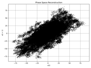
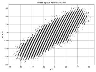
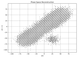
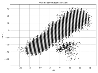
this, we employ phase space
reconstruction as illustrated in Figure 3.
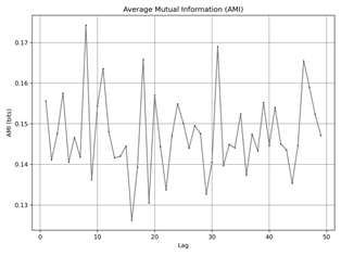
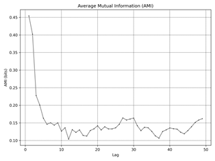
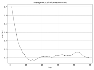
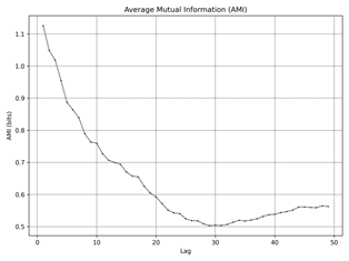
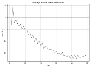
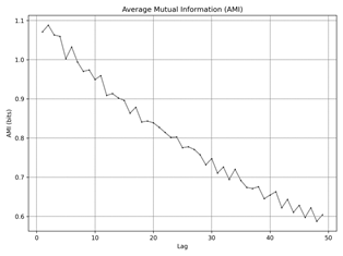
Figure 4
shows Average Mutual Information (AMI), measures the amount of information
shared between the time series and its lagged version as a function of lag.
This is crucial for identifying dependencies over time and helps in determining
the optimal time delay (τ) for reconstructing the phase space. The first
minimum of AMI indicates the lag at which the shared information is least,
suggesting the most independent state, and is used to set the optimal time
delay for further analysis. For dataset a) the optimal τ is 8.
This indicates that the time series shares the least information with its
lagged version at a lag of 8, suggesting this as the ideal time delay for phase
space reconstruction. For dataset b) the optimal τ is 4. A shorter time delay
implies that the system's dynamics change more rapidly compared to dataset a).
For dataset c)
similar to dataset a), the optimal τ is 8. For dataset d)
the optimal τ is 4, indicating rapid changes in system dynamics similar to
dataset b). For dataset
e) the optimal τ is 5, falling between the time delays
observed in datasets a), b), c), and d). The dataset’s f) optimal τ is 3,
suggesting very rapid changes in the system dynamics.
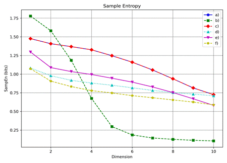
Figure
5 shows the Sample Entropy for different embedding dimensions (m), quantifying the complexity or irregularity
of the time series data. Higher Sample Entropy values indicate greater complexity and unpredictability.
By examining the Sample Entropy for varying
dimensions, we can identify the
optimal embedding dimension
for each dataset, which captures the system's
dynamics most effectively without over-embedding. It shows Sample Entropy quantifies the complexity or irregularity
of the time series data. The optimal embedding dimension (m) is found to
be a) m=10, b) m=4, c) m=10, d) m=4, e) m=5, f) m=3.
The optimal embedding dimension
is crucial for phase space
reconstruction, as it ensures that
the reconstructed state space retains
the essential characteristics
of the system's
dynamics while minimizing redundancy.
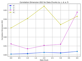
Figure
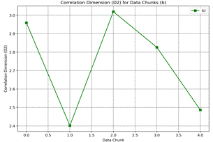
6 presents the correlation dimension (D2) for different data chunks. The correlation dimension provides insights into the
fractal nature of the data,
indicating the system's complexity. Higher values of the
correlation dimension suggest more complex
and higher-dimensional structures
within the time series data. These values indicate varying degrees of complexity across
the different datasets, with Dataset b) exhibiting significantly higher correlation dimensions, suggesting a more complex structure.
Figure 7
presents the Probability Density Function (PDF) of the normalized RPM data for
datasets a) to f). The PDF provides insights into the distribution of RPM
values, with peaks indicating the most frequently observed values. These peaks
suggest the dominant operating ranges of the RPM, highlighting where the system
tends to operate most frequently.
· Dataset a): Notable
peaks around [-55.90, -50.46, -45.02, -31.41, -25.97, -20.53, -12.37, -4.20,
6.68, 12.12, 20.29, 28.45]
· Dataset b):
Significant peaks around [-64.23, -57.43, -47.22, -40.42, -33.62, -26.82,
-23.42, -20.02, -6.42, 3.78, 13.98, 27.58, 34.38, 41.18]
· Dataset c): Major
peaks around [-55.90, -50.46, -45.02, -31.41, -25.97, -20.53, -12.37, -4.20,
6.68, 12.12, 20.29, 28.45]
· Dataset d): Distinct
peaks around [-76.59, -68.94, -61.30, -49.83, -42.19, -34.54, -26.89, -19.25,
-15.43, -3.96, 7.51, 18.98, 22.80, 34.27, 41.91, 45.74, 57.21]
· Dataset e): Prominent
peaks around [-57.48, -49.70, -41.93, -34.15, -25.97, -18.60, -10.83, -6.94,
0.83, 8.61, 16.38, 20.27, 28.05, 31.93, 39.71, 51.37, 55.26, 63.03, 70.81]
· Dataset f): Clear
peaks around [-125.68, -119.81, -113.95, -90.48, -72.89, -67.02, -49.42,
-31.83, -25.96, -20.10, 3.37, 15.10, 26.83, 38.56, 44.42, 50.29, 56.16, 62.02,
67.89, 79.62, 85.48]
These PDFs
(Fig.7) indicate the operational behavior and
dominant RPM ranges of the system, providing valuable insights into the
system's performance and stability.
|
|
|||
|
Fig. 5. Sample Entropy (SampEn) : idle a) ≈ 550 rpm, b) ≈ 1010 rpm, c) ≈2160 rpm, |
|
|
|
|
Fig. 6. Correlation
dimension (D2) for different data chunks: idle a) ≈ 550 rpm, |
|
Figure
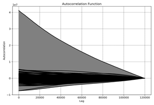
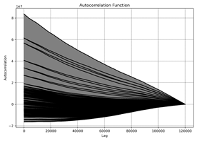
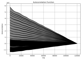
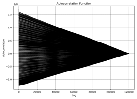
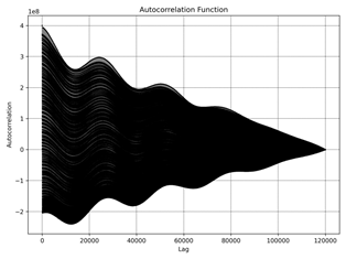
8 presents the Autocorrelation Function (ACF) for different datasets (a) to f)). The ACF measures the correlation of the time series
with its lagged versions. The decaying pattern observed in the ACF plots indicates the memory effect
in the RPM data, showing how past
values influence future values over
time.
Dataset a): The ACF
shows a gradual decay, indicating a long memory effect, where past values
significantly influence future values for a long duration.
Dataset b): The ACF
shows a faster decay, suggesting a shorter memory effect, with past values
having less influence over a shorter duration.
Dataset c): Similar
to dataset a), the ACF shows a gradual decay, indicating a long memory effect.
Dataset d):
The ACF shows a moderate decay, suggesting a moderate memory effect with a
balanced influence of past values on future values.
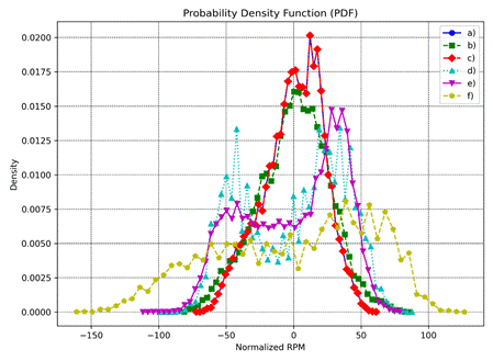
Fig.
7. Shows Probability Density Function (PDF): idle a) ≈ 550 rpm, b) ≈ 1010 rpm,
c) ≈2160
rpm, d) ≈ 3200 rpm,
full gas slope 12%, e) ≈ 2250 rpm; full gas slope 10%,
f) ≈2740 rpm
Dataset e): The ACF
shows a noticeable decay pattern, indicating a significant memory effect,
though not as long as datasets a) and c).
Dataset f): The ACF
shows a rapid decay, suggesting a very short memory effect, where past values
have minimal influence on future values.
Figure 9 presents
the Power Spectral Density (PSD) of the normalized RPM data across datasets a)
to f). The PSD plot offers a detailed view into the frequency domain
characteristics of the RPM data, elucidating how power is distributed across
various frequency components.
High Power at Low Frequencies: The PSD
reveals a higher concentration of power at low frequencies across all datasets,
suggesting that low-frequency components are predominant in the RPM signal.
This behavior indicates the presence of slow,
large-scale variations within the system's dynamics, which could be linked to
underlying processes or external influences that drive such fluctuations.
Decay of Power with Frequency: A
noticeable trend in the PSD is the general decay of power as frequency
increases. This pattern implies that high-frequency components possess less
energy and are consequently less influential in the overall behavior
of the RPM data. This decay is typical in systems where high-frequency noise or
rapid fluctuations are less dominant.
Distinct Peaks: The PSD
plots exhibit distinct peaks at certain frequencies, signifying specific points
where the system oscillates more intensely. These peaks are indicative of
resonant frequencies or harmonics, where the system's natural frequencies
align, resulting in amplified oscillations. Identifying these peaks is crucial
for understanding the resonant behavior and potential
instabilities within the system.
Comparative Analysis of Datasets: Each
dataset demonstrates a unique PSD profile, reflecting the variability in their
underlying dynamics. While some datasets show pronounced peaks at certain
frequencies, indicating stronger oscillatory behavior,
others may exhibit a more uniform distribution of power, suggesting different
operating conditions or external influences. Comparing these profiles allows
for a deeper understanding of how different conditions or regimes affect the
system's frequency response.
The PSD
analysis thus provides critical insights into the oscillatory behavior and frequency characteristics of the RPM data. By
understanding how power is distributed across frequencies, one can infer the
system's stability, identify dominant operational frequencies, and detect
potential resonances that could impact performance. This frequency domain
perspective complements time-domain analyses, offering a more comprehensive
understanding of the system's behavior.
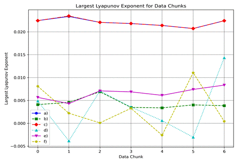
Figure 10 presents the Largest
Lyapunov Exponent (LE) calculated for different data chunks across datasets a)
to f). The Lyapunov exponent is a critical measure for identifying chaotic behavior within a system, where a positive LE indicates
chaos, and a zero or negative LE suggests stable or periodic dynamics. The
following parameters were used for the calculations:
Embedding dimension: 3
Time delay: 1`
Minimum
time separation: 2
Analysis by dataset:
a) The LE values range from 0.021 to
0.023, indicating significant chaotic behavior. The
system shows strong sensitivity to initial conditions, suggesting a highly
dynamic and unpredictable RPM behavior in this
dataset.
b) The LE values range from 0.003 to
0.007, indicating mild chaotic behavior. While still
positive, these lower LE values suggest a system with less pronounced chaos
compared to dataset a), but still exhibiting sensitivity to initial conditions.
c) The LE values range from 0.021 to
0.024, very similar to dataset a). This indicates significant chaotic behavior and strong sensitivity to initial conditions,
suggesting highly dynamic and unpredictable RPM behavior.
d) The LE values
range from -0.004 to 0.014, showing the widest variation among the datasets.
This indicates intermittent chaos, where some regions show strong chaotic
behavior (positive LE up to 0.014) while others display stable or potentially
periodic behavior (negative LE down to -0.004). This dataset suggests complex,
varying dynamics in the RPM behavior.
e) The LE values
range from 0.004 to 0.008, indicating consistent mild to moderate chaotic
behavior. All values are positive, suggesting that the system is consistently
sensitive to initial conditions, but with less intensity than datasets a) and
c).
f) The LE values
range from -0.003 to 0.01, showing significant variation similar to dataset d). This indicates intermittent chaos, with some data chunks
showing stable or potentially periodic behavior (negative LE) and others displaying
more pronounced chaotic characteristics (positive LE up to 0.01).
|
|
|
|
|
|
|
|
|
|
|
e) |
f) |
|
|
|
Fig. 8. Autocorrelation Function (ACF): idle a) ≈ 550 rpm, b) ≈ 1010 rpm, c) ≈2160 rpm, |
|
||
|
|
||
|
Fig. 9. Power Spectral Density (PSD): idle a) ≈
550 rpm, b) ≈ 1010 rpm, c) ≈2160 rpm, |
||
|
|
|
Fig. 10. Lyapunov exponent chunk: idle a) ≈
550 rpm, b) ≈ 1010 rpm, c) ≈2160 rpm, |
The analysis of Lyapunov exponents
provides valuable insights into the system's stability and predictability,
highlighting regions where chaotic behavior may
impact the RPM's performance. The varying degrees of chaos across different
datasets suggest that the internal combustion engine's RPM behavior
is highly dependent on specific operating conditions or parameters.
Datasets a) and c) show the most
pronounced chaotic behavior, while datasets b) and e)
display milder, but consistent chaos. Datasets d) and f) exhibit the most
complex dynamics, with intermittent chaos and periods of stability or potential
periodicity.
This comprehensive analysis across all
datasets reveals a rich tapestry of dynamic behaviors
in the internal combustion engine's RPM, ranging from strongly chaotic to
near-stable conditions, depending on the specific dataset and operating
parameters.
The analysis of the data presented in
Figures 1 through 10 reveals significant evidence of chaotic behavior across various operating conditions. Key findings
include:
1. Evidence of Chaos: The Largest
Lyapunov Exponent (LE) values consistently show positive values across all
datasets, ranging from 0.003 to 0.024. This indicates the presence of chaos in
the system, suggesting that the RPM is sensitive to initial conditions and
exhibits exponential divergence in trajectories over time.
2. Complexity of the System: The Sample
Entropy analysis identified optimal embedding dimensions ranging from 3 to 10
across different datasets. Higher values indicate greater irregularity and
unpredictability in the time series data. The correlation dimension values
varied significantly, with some datasets showing higher dimensions, suggesting
a more complex structure.
3. Optimal Time Delay: The Average Mutual
Information (AMI) analysis determined optimal time delays (τ) ranging from
3 to 8 across different datasets. This variation in optimal time delays
indicates that the system's dynamics change at different rates under various
operating conditions.
4. Memory Effects: The Autocorrelation
Function (ACF) analysis revealed varying degrees of memory effects across the
datasets. Some regimes exhibited long memory effects, where past values
significantly influence future values over an extended period, while others
showed short memory effects with rapidly decaying correlations.
5. Frequency Domain Insights: The Power
Spectral Density (PSD) analysis showed that low-frequency components dominate
the RPM signal across all datasets, indicating slow, large-scale variations in
the system. Distinct peaks at certain frequencies suggest the presence of
resonant frequencies or harmonics, which are critical for understanding the
system's oscillatory behavior and potential
instabilities.
6. Varying Chaotic Behavior:
The analysis revealed different levels of chaotic behavior
across operating conditions:
Datasets a) and c) (idle at ≈550
rpm and ≈2160 rpm) showed the most pronounced chaotic behavior
with LE values ranging from 0.021 to 0.024.
Datasets b) and e) (idle at
≈1010 rpm and full gas slope 12% at ≈2250 rpm) displayed milder but
consistent chaotic behavior.
Datasets d) and f) (idle at
≈3200 rpm and full gas slope 10% at ≈2740 rpm) exhibited the most
complex dynamics, with intermittent chaos and periods of stability or potential
periodicity.
Implications for System Monitoring and Control:
1. Challenges in Long-Term Prediction:
The chaotic nature of the system makes long-term precise predictions inherently
challenging. Small differences in initial conditions can lead to vastly
different outcomes over time.
2. Importance of Short-Term Forecasting:
While long-term predictions may be unreliable, short-term forecasting can still
be valuable. Understanding the system's immediate dynamics can help anticipate
short-term changes and inform decision-making.
3.
Advanced Control Strategies: The varying degrees of chaos across
different operating conditions suggest that adaptive control strategies are
necessary. These strategies should account for the system's nonlinear dynamics
and be able to adjust to different chaotic regimes.
4. Resonance Management: The PSD analysis
revealed distinct peaks at certain frequencies. Managing these resonant
frequencies could be crucial for maintaining system stability and optimizing
performance.
5.
Real-time Monitoring: Given the system's sensitivity to initial
conditions and its complex dynamics, real-time monitoring of the RPM becomes
essential for detecting and responding to potential instabilities or
performance issues.
4. DISCUSSION
The
analysis, employing various techniques from chaos theory and nonlinear
dynamics, provides a detailed picture of the engine's behavior
under various operating conditions. Results show that RPM dynamics exhibit
different levels of chaos and complexity depending on the engine's operating
regime, with implications for engine design, control, and diagnostics.
To
facilitate further research and collaboration, the authors have shared the
original datasets and analyzed Python code [15]. This
openness allows for verification of results, further exploration of complex
processes in internal combustion engines, and investigation into the influence
of chaotic dynamics versus random fluctuations on engine behavior.
The
authors welcome further discussion and collaboration to deepen our
understanding of these complex dynamics and their implications for engine
performance, efficiency, and control strategies. This study builds upon
previous work in the field and extends the application of chaos theory to the
analysis of RPM fluctuations, providing a comprehensive framework for analyzing engine dynamics that could be applied to various
engine types and operating conditions.
By
combining high-precision measurements with advanced analytical techniques, this
research opens new avenues for understanding and optimizing internal combustion
engine performance, highlighting the importance of considering nonlinear and
chaotic behaviors in engine analysis and design.
5. CONCLUSIONS
The
analysis of the rotational speed data reveals significant chaotic behavior in the internal combustion engine's RPM across
various operating conditions:
1. Lyapunov
Exponents: highest 0.024 (idle at ≈550 rpm and ≈2160 rpm),
indicating strong chaos and high sensitivity to initial conditions; lowest:
-0.004 (idle at ≈3200 rpm), suggesting occasional periods of stability.
The predominantly positive Lyapunov Exponents confirm the presence of chaos in
the system.
2. Optimal Time
Delay (τ): ranges from 3 to 8 across datasets, shortest (τ = 3) at
full gas, slope 10%, ≈2740 rpm, indicating rapid changes in system
dynamics, longest (τ = 8) at idle, ≈550 rpm and ≈2160 rpm,
suggesting slower changes in system dynamics.
3. Optimal
Embedding Dimension (m): ranges from 3 to 10 across datasets, highest (m =10)
at idle, ≈550 rpm and ≈2160 rpm, suggesting high system complexity,
lowest (m =3) at full gas, slope 10%, ≈2740 rpm, indicating simpler
system dynamics.
4. Power Spectral
Density: all datasets show higher concentration of power at low frequencies
(0.1 Hz to 0.5 Hz), indicating dominance of slow, large-scale fluctuations.
References
1.
Boeing Geoff. 2016. "Visual analysis of
nonlinear dynamical systems: chaos, fractals, self-similarity and the limits of
prediction". Systems 4: 37. DOI: 10.3390/systems4040037.
2.
Stewart Ian. 2000. "The lorenz
attractor exists". Nature 406: 948-949. DOI: 10.1038/35023206.
3.
Wendeker Miroslaw,
Jacek Czarnigowski, Grzegorz Litak, Kazimierz Szabelski.
2003. "Chaotic Combustion in spark ignition engines". Chaos
Solitons & Fractals 18(4): 803-806. DOI: 10.1016/S0960-0779(03)00031-6.
4.
Huanyu Di, Shen Tielong. 2018. "Experimental analysis of chaotic
property of in-cylinder combustion of si
engine." 37th Chinese Control Conference (CCC): 7907-7911. Wuhan,
China. DOI: 10.23919/ChiCC.2018.8483466.
5.
Lima, Thyago L. de V., Abel C.L. Filho,
Francisco A. Belo, Filipe V. Souto, Thaís C.B. Silva, Koje
V. Mishina, Marcelo C. Rodrigues. 2021. "Noninvasive
methods for fault detection and isolation in internal combustion engines based
on chaos analysis". Sensors 21(20): 6925. DOI: 10.3390/s21206925.
6.
Grabar Ivan, Andrii Ivanchenko, Volodymyr Lomakin,
Dmytro Kalinkin, Oleksandr Kuharchuk.
2010. "Hardware and software complex for analyzing
the operation of the MeMZ-2457 engine by rotation frequency fluctuation". Scientific
Notes of the National Technical University 28: 151-156.
7.
Lomakin Volodymyr. 2018. "Decreasing of
speed fluctuation of internal combustion engine by improving the flywheel
design". Doctoral dissertation. Available at: http://diser.ntu.edu.ua/Lomakin_dis.pdf.
8.
Takens Floris.
1981. "Detecting strange attractors in turbulence". Dynamical
Systems and Turbulence 898: 366-381.
10.
Wolf Alan, Jack B. Swift, Harry L. Swinney, John A. Vastano.
1985. "Determining Lyapunov exponents from a time series". Physica
D: Nonlinear Phenomena 16(3): 285-317. DOI: 10.1016/0167-2789(85)90011-9.
11.
Grassberger Peter, Itamar Procaccia.
1983. "Measuring the strangeness of strange attractors". Physica
D: Nonlinear Phenomena 9(1-2): 189-208. DOI: 10.1016/0167-2789(83)90298-1.
12.
TheilerJames, Stephen Eubank, André Longtin, Bryan Galdrikian,
J. Doyne Farmer. 1992.
"Testing for nonlinearity in time series: the method of surrogate
data". Physica D: Nonlinear Phenomena 58(1-4): 77-94. DOI: 10.1016/0167-2789(92)90102-S.
13.
Chaotic-engine-rpm-analysis project with raw
data. Available at: https://github.com/VD45/chaotic-engine-rpm-analysis.
14.
Numpy 2.0. The
fundamental package for scientific computing with Python. Available at: https://numpy.org/.
15.
Pandas. The fast, powerful,
flexible and easy to use open source data analysis and manipulation tool, built
on top of the Python programming language. Available at: https://pandas.pydata.org/.
16.
SciPy.
Fundamental algorithms for scientific computing in Python. Available at: https://scipy.org/.
17.
Matplotlib. Visualization with
Python. Available at: https://matplotlib.org/.
18.
SciKit. Machine
Learning in Python. Available at: https://scikit-learn.org/stable/.
19.
Python Programming Language. Available at: https://www.python.org/.
Received 10.01.2025; accepted in revised form 05.04.2025
![]()
Scientific Journal of Silesian
University of Technology. Series Transport is licensed under a Creative
Commons Attribution 4.0 International License
