Article citation information:

Gruchot, A., Zydroń, T. Assessment of the acoustic climate on the example of the road in Michałowice (Poland). Scientific Journal of Silesian University of Technology. Series Transport. 2025, 127, 103-128. ISSN: 0209-3324. DOI: https://doi.org/10.20858/sjsutst.2025.127.7

Andrzej GRUCHOT[1], Tymoteusz ZYDROŃ[2]

ASSESSMENT OF THE ACOUSTIC CLIMATE ON THE EXAMPLE OF THE ROAD IN MICHAŁOWICE (POLAND)

Summary. The aim of the research was to assess the acoustic climate along the DK7 national road in Michałowice (Kraków district, Poland). The climate assessment was carried out during the period from September to May at two measurement sites located at a distance of 11.5 and 27.0 m from the road. The scope of the study included measuring the intensity of noise, recording the number of light and heavy vehicles, measuring the temperature of as well as air and the type of precipitation. The results of noise intensity measurements showed numerous cases of exceeding the permissible equivalent noise level for single-family housing areas. The machine learning methods used showed that the noise level was influenced by air temperature, snowfall, and plant vegetation. Significantly lower values of the equivalent noise level were obtained on weekends, indicating that commercial road traffic prevailed in the analyzed road section.

Keywords: road traffic noise, noise pollution, equivalent sound pressure levels, atmospheric conditions

1. INTRODUCTION

Noise and its level have become one of the factors that increasingly characterize the areas where people live, work, or relax. Noise is the biggest problem for city dwellers, but it is also recorded in rural areas, as well as in city parks and even in national parks and reserves. Long-term exposure to unwanted sounds results in hearing damage and deterioration of mental health and general health.

Noise is defined as unpleasant and undesirable sounds with frequencies from 16 Hz to 16 kHz and with an intensity that causes nuisance to the surroundings [13]. Noise is estimated to be the world's biggest problem after air pollution. This pollution comes from the places where people live and work. The sources of noise are mainly industrial and service activities, as well as transport. Sound, in physical terms, is the mechanical deformation of an elastic medium (such as a gas or liquid) moving in the form of a wave. Sound can be described as the propagation of small pressure disturbances and density fluctuations in such a medium. The basic quantity that describes sound is its frequency and the amplitude of the sound pressure.

The definition of noise contained in the Environmental Protection Law [13] does not include the important psychophysiological aspect due to which the specific concept of "sound" is transformed into the concept of "noise". Directive 2002/49/EC [12] treats the concept of noise more broadly, stating that "environmental noise" means unwanted or harmful sounds caused by human activities. Depending on the source of origin, a distinction is made between traffic noise (road or street noise, aircraft, railway, and tram noise), industrial noise (metal and wood processing, construction, ventilation, and air conditioning installations), and municipal noise (catering establishments, concerts, sports competitions).

Road noise is estimated to be the most common type of noise. According to the Strategic Noise Mapping database, one in five people in Europe are exposed to chronic noise levels that can cause adverse health effects. Around 95 million people in the European Union are estimated to be exposed to harmful levels of road noise, and at least 20% of the urban population is exposed to noise levels considered harmful to health. At least 18 million people are very irritated and 5 million have severe sleep disturbances due to long-term exposure to transport noise. Furthermore, it is estimated that long-term exposure to transport noise causes approximately 11000 premature deaths and, 40000 new cases of coronary heart disease [53]. In Iceland, Norway, Switzerland, and Turkey, one in four households reports being bothered by the noise of neighbors or from the street, with the proportion of the population complaining about noise ranging from 12% (in Hungary, Iceland, Ireland, and Norway) to 31% (in Cyprus and Romania). The World Health Organization (WHO) estimates that approximately 40% of the population is exposed to road noise exceeding 55 dB, 20% are exposed to noise exceeding 65 dB during the day, and more than 30% are exposed to noise exceeding 55 dB at night [56]. Road noise is also closely related to air pollution and its impact on human health [3, 17, 42], as well as to animals living on land and in water [44, 26]. Long-term exposure to noise is harmful to physical and mental health. Excessive noise levels cause sleep disorders, which in turn leads to cardiovascular diseases, as well as irritation, learning difficulties, hearing impairment and tinnitus, chronic fatigue, irritability, stress, loss of concentration and other diseases [2, 20, 52].

Road noise is one of the main factors that degrade the environment, and its impact is increasing due to the construction of new roads and communication routes. Therefore, the effects of its impact are felt by an increasing number of residents. The level of road noise is influenced by the density of roads and streets in urban areas, and outside cities, highways and expressways, as well as national and some provincial roads. The condition of the road surface and the means of transport on the roads are also important. The noise caused by the engine, the rolling noise (contact of the tire with the ground), and the aerodynamic noise (turbulent air flow around the body of the car) are important factors influencing the noise level. In the case of heavy vehicles, there are also vibrations of some elements (e.g., vibrations of semitrailers or containers) when driving on uneven surfaces.

The type of noise source will determine the acoustic climate of a given place, which is most often characterized by the sound level occurring in a given area. Acoustic climate is a set of acoustic phenomena that occur in the environment and are caused by noise coming from sources located in this environment. Acoustic climate is assessed using the sound level of all sources that cause it in a given environment. The harmfulness of noise depends on the level of sound pressure and the duration of exposure, that is, the so-called noise dose [7]. Acoustical climate, especially under local conditions, is characterized by strong changes in time and space. It depends mainly on the degree of saturation of a given environment with devices and vehicles, as well as the urban layout characterizing the local environment and the layout of housing estates with green areas, communication system, commercial and service facilities and production plants. Therefore, environmental noise is attracting more and more attention and is regulated by an increasingly demanding legal framework because its effects on the population are worrying [25, 40].

In Poland, road noise measurements are performed as part of environmental monitoring or control and by road management institutions. Based on the results of noise level measurements, acoustic condition assessments are carried out. Long-term trends in environmental noise in Poland indicate an increase in traffic noise, especially road and aircraft noise. The increase in the risk of road noise in recent years is mainly related to the construction of new roads and elements of the road infrastructure and the rapid increase in the number of vehicles [19].

The monitoring of noise level showed that in 2020, road noise in Poland was a threat primarily in urbanized areas and was felt by an increasing number of residents [20]. Of almost 200 km of roads, only 4% of roads had road noise emissions in the range of up to 60 dB, that is, emissions that did not exceed allowed sound levels during the day in residential areas adjacent to the roads. The highest percentage of streets with exceeded noise emissions was found in the cities of the Lower Silesian, Lubuskie, Lesser Poland and Podlaskie voivodeships (100% each) and the West Pomeranian voivodeship (99%). The lowest percentage was in the cities of the Lublin Voivodeship (69%) and the Warmian-Masurian Voivodeship (71%) [20]. The research results have shown that the greatest impact of traffic noise on the acoustic climate occurs 200-300 m from the road, and the nuisance of traffic noise reaches a distance of approximately 500 m from the road [5]. The level of traffic noise, both in cities and on communication routes in non-urban areas, is determined by many factors, including vehicle traffic intensity, the percentage share of trucks in the traffic flow, the speed of vehicles, the location of the road and the type of surface, the condition of the road, the topography and types of buildings, the driving style of drivers.

The aim of the study was to evaluate the acoustic climate on Krakowska Street in Michałowice (Kraków district, Poland) along the DK7 national road. The evaluation was based on the calculated equivalent noise level calculated for the time of day.

2. CHARACTERISTICS OF THE RESEARCH SITE

The research was carried out in the Michałowice in the Lesser Poland Voivodeship, Kraków District (Fig. 1). The measuring points were located on Krakowska Street, which is part of National Road DK7. The permissible speed of vehicles on the analyzed road section is
50 km×h^-1.

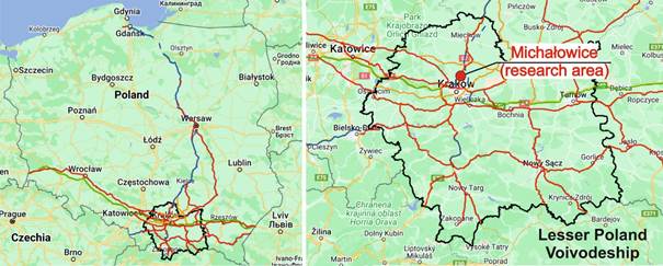
Fig. 1. Location of Michałowice and the route of the DK7 road (own study after [54])

In the research section, the DK7 road has one lane in each direction (Fig. 2). The measurement sites were located on the western side of the road. On the eastern side of the road, there is a gravel bicycle path, which is separated from the road by a 0.5 m wide shoulder. On the opposite side of the measurement site, there is a steep exit from Spokojna Street. This may generate increased noise levels as many drivers have difficulty exiting this street. A characteristic element of the road in the research section was a speed camera. Despite the correct marking of the speed camera (vertical road sign D-51), its frequent activation indicates that the speed limit has been exceeded. You can also notice that drivers slow down and then accelerate in front of a speed camera, which also affects the noise level. A certain limitation to this behavior of drivers is the pedestrian crossing located 50 m behind the speed camera towards Warsaw.

National Road DK7 in the section where the research section is located is straight and flat, and its condition can be assessed as very good. The asphalt was replaced in 2017, so there were no defects that would generate additional noise. Approximately 250 m south of the research section, there is a traffic light that causes traffic jams during heavy traffic. Such situations are mainly observed in the morning and during heavy tourist traffic. On the western side of the road, there is a drainage ditch approximately 1 m deep. The ditch is regularly mowed and is kept in good condition. Next, there is a 2.0 m wide pedestrian sidewalk. The traffic on the road is small and did not affect the measurement results.

3. METHODOLOGY

The noise intensity was measured using a Voltcraft SL-451 decibel meter, which met the requirements of class 2 [38]. The measurement accuracy was 1.4 dB and the supported frequency range was 31.5 to 8000 Hz. The sonometer's microphone was protected by a sponge so that the wind did not cause any disturbances in the measurement.

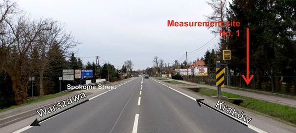
Fig. 2. Road infrastructure in the research section (photo by D. Wywiał)

The measurement sites were located on a private plot, located directly next to the DK7 road (Fig. 3). The measurement sites were located at two different distances from the road axis. The site No. 1 (Fig. 4a) was located 11.5 m from the road axis, directly behind the metal mesh fence. The sonometer was installed at a height of approximately 0.5 m above the ground surface. Measurement site No. 2 (Fig. 4b) was located at a distance of 27.0 m from the road axis at a height of 1.5 m on the wall of a single-family building. In this case, there was loose vegetation between the DK7 road and the sonometer. Near the fence there were thujas up to 0.5 m high, then tall pines without branches up to 2.0 m high, and then vegetation up to 3.0 m high.

Noise intensity measurements were carried out in six 5-day measurement cycles in September, October, and November and in January, April, and May. At site 1, measurements were performed on Mondays, Thursdays, and Saturdays, and at site 2 on Tuesdays and Fridays. The tests started at 7:00, 12:00 and 17:00 and lasted 60 minutes with the sound level recorded every 1 second. Additionally, the number of passing cars, divided into light and heavy, as well as the temperature of the air and the type of precipitation, were recorded. The research was carried out regardless of weather conditions.

The data collection period was limited to the time of day (6:00-22:00) because it was expected that peak hours of morning, afternoon, and evening traffic would fall during this period. The study assumed that noise levels during the day were more critical than noise levels at night.

The currently applicable legal acts regulating the permissible levels of noise in the environment are the regulation of the Minister of the Environment of October 8, 2012, amending the regulation on permissible noise levels in the environment [14] and the announcement of the Minister of the Environment of October 15, 2013 with respect to the announcement of the uniform text of the Minister of the Environment on permissible noise levels in the environment [15]. According to this legal act, the permissible levels of environmental noise caused by roads or railway lines, expressed in equivalent sound levels, range from 50 to 68 dB during the day (16 hours of reference time) and from 45 to 60 dB at night (8 hours). Table 1 presents the permissible levels of environmental noise caused by individual groups of noise sources, excluding noise caused by aircraft take-offs, landings, and flights, as well as power lines, expressed in the LAeqD and LAeqN indicators [14]. These indicators apply to the establishment and control of conditions of use of the environment in relation to one day.

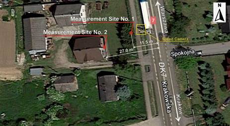
Fig. 3. Location of measurement sites in relation to the DK7 road (own study after 54])

a) measurement site No. 1

b) measurement site No. 2

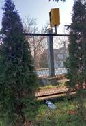
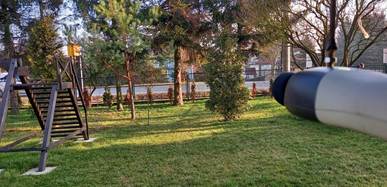
Fig. 4. View from the measurement sites onto the DK7 road (photo by D. Wywiał)

The acoustic climate is determined using acoustic indicators of long-term external noise and short-term acoustic indicators, corresponding to an equivalent noise level, and associated with general discomfort and disturbances of sleep. The equivalent noise level is given in decibels and is the value of the sound pressure level of a continuous steady sound, corrected according to the frequency characteristic A, which in a specific reference time interval is equal to the mean square of the sound pressure of the analyzed sound with a level varying in time [13]. Most often, the equivalent sound level is given for the time of day (reference time interval of 16 hours - from 6:00 to 22:00) and night (reference time interval of 8 hours – from 22:00 to 6:00). The equivalent noise level is expressed by the formula according to [39]:

(1)

where n – number of measurements, LA - the average sound level A that occurs during measurement.

Tab. 1

Permissible levels of environmental noise caused along roads and railway lines
(own study after [15])

No	Type of terrain	Permissible noise level in [dB] for roads or railway lines
		reference time interval
		time of day LAeq D	night time LAeq N
1	a) Protection zone "A" of the health resort b) Hospital areas outside the city	50	45
2	a) Areas of single-family housing development b) Development areas related to permanent or temporary stay for children and young people c) Areas of social welfare homes d) Hospital areas in cities	61	56
3	a) Areas of multifamily housing development and collective housing b) Farm development areas c) Recreational and relaxation areas d) Residential and service areas	65	56
4	Areas in the inner-city zone of cities with more than 100,000 inhabitants. inhabitants	68	60

For the tests carried out, the equivalent noise level was determined for the time of day separately for each of the three measurement hours and then as a total value for the three measurement hours. For the research area in question, according to [15], the acceptable noise level in the environment for the day is 61 dB and for the night it is 56 dB.

Measurement results were subjected to statistical analysis. The influence of the factors analyzed (day and measurement time, temperature, traffic intensity of light and heavy vehicles) on the recorded values of the equivalent noise level was determined. To verify the normality of the distribution, the data were independently subjected to the Shapiro-Wilk test and then the U-Mann-Whitney and Kruskal-Wallis tests were used. Later in the analysis, machine learning methods were used to determine the importance of each of the measured (or recorded) factors. The Ridge Regression with cross validation (with l2 regularization), support vector machine, multilayer perceptron, k-nearest neighbor and ensemble method, bagging regressor with the Decision Tree Regressor as the base estimator were used. To reduce the over- or under-fitting of the models, the data were split into train and test sets with proportions of 75% and 25%. Qualitative factors (hour of measurement, weather type) were transformed using a one-zero numeric array. Instead of the number of months, the cyclical features were created using the cosine function, and the months were classified as vegetative or nonvegetative. The days were transformed into weekday or weekend days. The additional factor used in the analysis was the total number of vehicles, in which each lorry was equivalent to 2.5 passenger cars. The use of machine learning models allowed us to explain the role of the set of independent factors in the dependent factor (equivalent to the continuous sound level). To assess the importance of each factor, Shapley values were used. The coding of data was used in Python using pandas [34], numpy [22] libraries. Data transformation was performed using the sklearn library [37] and the feature engine [18] libraries, while models were implemented with the use of the sklearn library. The Shapley values were determined using the SHAP library [29, 30]. Other statistical tests were used using the SciPy library [49], and results visualizations were prepared using matplotlib [24] and seaborn libraries [50].

4. RESEARCH RESULTS AND THEIR ANALYSIS

For the six measurement cycles carried out, the noise level directly from the sonometer measurements ranged from 41 dB to 111 dB, and its highest values were recorded in January (Fig. 5). The recorded sound intensity range ranged from the sound level of a conversation to that of a crowded street. Due to the requirements established by the regulatory regulations, a further analysis of the results obtained was carried out for the value of the equivalent noise level calculated according to (1) for each hour of a given measurement cycle. Table 2 shows the results of the calculation of the equivalent noise level calculated for the measurement hours and the total noise level calculated for the three measurement hours. The table shows the results of calculations and carried out at measurement site No. 2 in italics, and the minimum and maximum values of the equivalent noise level for individual measurement hours are marked in colors.

During the study period, 884 to 1508 light vehicles and 14 to 170 heavy vehicles were registered during one hour of measurement. There was a clear downward trend in the number of heavy vehicles during nonwork days (weekends, holidays), which was the result of applicable road traffic regulations.

Tab. 2

Summary of calculations of the equivalent noise level, number of vehicles,
temperature, and type of precipitation for each measurement cycle

Date of the measurement cycle		Equivalent noise level [dB] for:				Number of vehicles [pcs]		Tempera-ture [°]	Type of precipitation
		hours			day	light	heavy
date	Day	7:00-8:00	12:00-13:00	17:00-18:00
31/08 – 5/09	Mo	64.8	65.4	67.5	65.9	3575	407	17–19	lack
	Tu	66.7	68.7	64.9	66.8	3227	357	15–17	rain
	We	66.7	64.7	66.1	65.8	3720	418	16	lack
	Fr	65.3	64.2	63.0	64.2	3782	382	16–23	lack
	Sa	63.9	61.9	61.8	62.5	3592	52	17–24	lack
28/09 – 3/10	Mo	69.8	67.7	66.5	68.0	3362	440	5–13	lack
	Tu	65.9	65.0	65.5	65.5	3374	439	12–16	lack
	We	67.5	72.1	77.4	72.3	3462	383	11–13	rain
	Fr	64.8	65.4	65.1	65.1	3827	385	11–18	rain - none
	Sa	65.4	64.7	65.0	65.0	3690	66	12–24	lack
2/11 – 7/11	Mo	68.6	70.5	68.5	69.2	2821	376	5–12	fog - rain
	Tu	65.8	65.0	65.1	65.3	3212	422	11–15	lack
	We	69.5	67.7	74.7	70.7	3101	449	4–8	lack
	Fr	66.7	66.5	66.5	66.6	3752	390	5–11	lack
	Sa	67.2	67.2	67.3	67.2	3131	128	8–12	fog - none
11/01 – 16/01	Mo	70.2	69.2	69.7	69.7	2840	527	(-3)–2	lack
	Tu	68.9	67.9	66.4	67.7	3270	478	(-3)–4	snow
	We	68.5	69.9	66.4	68.3	2880	517	0–1	snow
	Fr	69.7	67.7	65.8	67.7	3299	448	(-3)–0	snow
	Sa	66.0	67.1	64.1	65.7	2791	165	(-5)–(-2)	snow
12/04 – 17/04	Mo	67.2	65.4	64.8	65.8	2723	1141	11–18	lack
	Tu	68.4	68.6	71.1	69.3	2394	680	4–10	lack
	We	70.4	66.8	70.8	69.3	2571	644	2–49	lack
	Fr	70.5	70.0	69.4	70.0	2658	670	3–4	lack
	Sa	67.5	68.0	66.1	67.2	2277	235	4–6	rain
26/04 – 1/05	Mo	67.9	66.5	66.0	66.8	2975	704	5–11	lack
	Tu	67.4	64.1	66.9	66.1	2895	706	6–12	lack
	We	68.0	65.6	64.6	66.1	2898	643	13–21	none - rain
	Fr	65.3	65.2	63.2	64.6	3283	588	15–20	rain - none
	Sa	65.8	64.2	62.8	64.2	2502	123	11–16	rain - none
Colors: – minimum values; – maximum values; In italics, marked results of measurements carried out at measurement site No. 2

The results obtained from the calculations of the equivalent noise level indicate slight differences between its values for the adopted measurement hours. It was also not found that any of the measurement hours was dominant in the conducted research (Fig. 6a). The minimum values of the equivalent noise level on measurement days ranged from approximately 62 to 65 dB and occurred most often at 5 p.m. on Friday or Saturday. However, the maximum values ranged from 68 to more than 77 dB. Values above 75 dB can be considered incidental, resulting from the passage of emergency vehicles with the sound signal.

However, the total values of the equivalent noise level calculated from three measurement hours ranged from nearly 63 to more than 77 dB (Fig. 6b). These values differ slightly from the values obtained for individual measurement hours and are therefore considered reliable in further analysis. The values obtained indicate that for each of the 30 measurement days, the equivalent noise level for the time of day was exceeded according to [17].

In assessing the state of the acoustic climate, in terms of road noise, a traffic noise hazard scale, which is auxiliary to the legal criteria, is often used, using subjective assessments. The Polish National Institute of Hygiene (PZH) developed, based on survey research, a subjective external scale for the time of day of traffic noise annoyance [27]. On this basis, it can be concluded that in the studied area, 28 out of 30 measurement days were days with high noise nuisance. On the remaining two days, very high noise was observed (Table 3). A similar finding was found for acoustic comfort. According to the scale presented in Table 3, there are mainly conditions corresponding to average noise hazard and high noise hazard [45].

a) January, Monday	b) January, Tuesday
c) January, Thursday	d) January, Friday
e) January, Saturday

Fig. 5. Point cloud for the third measurement cycle at site 1 (a, c, e) and site 2 (b, d)

a) hourly values	b) total values

Fig. 6. Changes in the equivalent noise level for the time of day during measurement cycles (the red line marks the permissible value [15])

Tab. 3

Summary of the number of days with a specific degree of noise nuisance and comfort

Parameter			Number of days
			Monday	Tuesday	Wednesday	Friday	Saturday
Noise nuisance for the noise level according to the Polish National Institute of Hygiene [27]
Little
Mean
Big			6	6	4	6	6
Very big					2
Acoustic comfort for the time of day [45]
Full acoustic comfort
Average acoustic conditions
Average noise hazard			6	6	4	6	6
High noise hazard					2

4.1. The Influence of distance from the road

The distance of both measurement sites from DK7 had little impact on the total values of the equivalent noise level (Fig. 6b). For individual measurement cycles, it was found that for most of the tests carried out, the maximum and minimum values of the equivalent noise level were obtained at measurement site No. 1, i.e. directly at DK7. It should be clearly indicated that in the case of the measurement cycle carried out in September and April, the maximum values of the equivalent noise level were obtained at measurement site No. 2 - 66.8 dB and 70.0 dB, respectively. Despite the nearly 16-meter difference in the distance between the measurement sites and the existing vegetation, the minimum values of the equivalent noise level at measurement site No. 2 were obtained only for the measurement cycle conducted in November. This value was slightly over 65 dB. It should be clearly indicated that the coniferous vegetation between the measurement sites did not limit the spread of noise from the DK7 road. Based on the results of the measurements obtained, it would be worth considering changing the development of this area by planting deciduous plants, which would reduce the nuisance associated with exceeding the noise level at least during the growing season [31, 32].

The comparison of the equivalent noise level recorded at both measurement sites could have been subject to an error resulting from the change of the measurements at these sites by at least 24 hours. However, the number of cars, which is the main factor causing noise, allows such comparisons to be made. When comparing the values of the equivalent noise level obtained at measurement site No. 2 on Tuesdays and Fridays with the results from measurement site No. 1 on Monday and Thursday, respectively, minor discrepancies were found. The differences between Tuesday and Monday ranged from -4.0 to 3.6 dB (-6 to 5%), and between Friday and Thursday from -12.3 to 0.3 dB (-16 to 0.1%).

4.2. The Influence of the number of vehicles

The impact of vehicle traffic and its relationship with road geometry and traffic organization on the noise level in its surroundings is the subject of many studies conducted around the world [1, 47]. These studies often involve the development of new or improved models and methods for forecasting noise in the vicinity of roads, which are necessary to control the acoustic climate and prevent the impact of excessive noise levels. The basic traffic parameters that influence road noise are: traffic intensity, vehicle speed, and share of heavy goods vehicles. The type of surface on which vehicles drive and the geometry of the road, mainly its longitudinal inclination, also have a significant impact on noise emission [6].

The analysis of the impact of the number of passing vehicles on the noise level was carried out with a distinction between light and heavy vehicles (Table 2, Fig. 7). Light vehicles were assumed to include passenger cars and delivery vans that do not exceed 3.5 tons of total weight, as well as motorcycles and mopeds. The number of light vehicles registered in each measurement hour ranged from 471 to 1,508 units, with an average of 970 units and a standard deviation of 198 units. The lowest values were recorded from 7:00 to 8:00 on Saturdays and the highest from Monday to Friday, from 17:00 to 18:00. However, the number of heavy vehicles ranged from 98 to 572 units with an average of 175 units and a standard deviation of 67 units from Monday to Friday. On Saturdays, due to applicable road traffic regulations, the number of heavy vehicles decreased significantly and ranged from 14 to 93 vehicles, with an average of 43 vehicles and a deviation of 22 vehicles. The number of registered vehicles resulted in equivalent noise levels ranging from 65 to 75 dB in November and from 62 to 69 dB in September. Thus, when the number of vehicles was reduced, the noise level remained above the allowed values.

The total number of vehicles during the three measurement hours ranged from 2,512 units (Saturday, April) to 4,212 units (Friday, October), with an average number of 3,575 vehicles (standard deviation 416). The number of heavy vehicles ranged from 52 to 1,141 units during the measurement day, which represented just over 1% (Saturday, September) to nearly 30% (Monday, April) of all vehicles (Table 1). The smallest number of heavy vehicles, 52 to 235 vehicles, was recorded on Saturday and from Monday to Friday it was from 123 to 1,141 vehicles.

However, despite significant fluctuations in the number of vehicles, there was no significant reduction in the value of the equivalent noise level with a reduction in their number. The average value of the equivalent noise level from Monday to Friday for six measurement cycles was close to 68 dB. However, on Saturday, where the smallest number of vehicles, mainly heavy vehicles, was found, the average equivalent noise level was just over 65 dB. On the other hand, the highest number of heavy vehicles was recorded mainly on Thursdays, and therefore it was the day with the highest equivalent noise level, exceeding 70 dB. Therefore, it can be concluded that an increase in the number of heavy vehicles increases the equivalent noise level.

4.3. The influence of atmospheric factors

Air temperature has a significant impact on the acoustic properties of the atmosphere. An increase in temperature usually results in an increase in the speed of sound in air, which can have consequences on the noise level in a given location. The increase in temperature also affects sound dissipation processes. In warmer air, there may be differences in air density and speed at different altitudes, which can lead to more complicated sound propagation trajectories.

The amplitude of temperature fluctuations for 5-day cycles of noise intensity measurements performed from late summer to spring was 29°C. The air temperature during this time decreased from 24°C in September 2020 to -5.0°C in January and increased to 21°C at the end of April. The average equivalent noise level for the entire measurement cycle ranged from 65 dB in September through 67 dB in October to 68 dB in November, January, and the first half of April and to 66 dB at the end of April.

In September, the air temperature ranged from 15°C to 24°C with changes in the equivalent noise level for individual measurement hours from 61.8 to 68.7 dB, in October the temperature ranged from 5°C to 24°C with changes in the equivalent noise level from 64.7 to 77.4 dB (Table 1, Fig. 8). A similar range of equivalent noise level was found in November (from 65.0 to 74.7 dB) at an air temperature of 4°C to 15°C. It can therefore be concluded that at a similar or lower air temperature compared to September, an increase in the recorded noise level was recorded from 3 dB to 9 dB. In January, negative air temperatures were recorded (from -5.0°C to 4.0°C) with a lower noise level of 1 dB to 4 dB (range was from 64.1 dB to 70.2 dB) were recorded compared to November. However, already at the beginning and end of April, when the temperature ranged from 2°C to 18°C and from 6°C to 21°C, the equivalent noise level compared to January was at a similar level (from 62.8 dB to 68.0 dB) or decreased and ranged from 62.8 dB to 68.0 dB. The analysis shows that temperature fluctuations did not cause significant changes in the equivalent noise level.

a) measurement site No. 1, hour 7:00-8:00	d) measurement site No. 2, hour 7:00-8:00
b) measurement site No. 1, hour 12:00-13:00	e) measurement site No. 2, hour 12:00-13:00
c) measurement site No. 1, hour 17:00-18:00	f) measurement site No. 2, hour 17:00-18:00

Fig. 7. Comparison of changes in the number of light and heavy vehicles in relation to changes in the equivalent noise level during measurement cycles

The analysis of the relationships obtained between air temperature and the equivalent noise level did not show a significant relationship between air temperature and noise level (Fig. 8). Air temperature changes resulting from the time of day (morning, noon, afternoon) during measurement cycles do not significantly affect the equivalent noise level. However, it should be clearly noted that the equivalent noise level increased from Monday to Thursday and then decreased from Friday to Saturday). However, this was more due to the number of vehicles than to weather conditions, especially the temperature.

As noted above, long-term exposure to noise can have a negative impact on people's mental and physical health. Therefore, understanding the effect of temperature on equivalent noise levels is important for developing effective noise management strategies and improving the quality of life of residents. Therefore, it should be noted that when recording the noise intensity, in addition to the air temperature, the air humidity level should also be recorded. It can be assumed that air humidity in connection with air temperature would indicate to a greater extent the dependence of noise on the atmospheric conditions prevailing around the measurement site.

During 30 days of observations, there were 22 days in which no rain was observed or rainfall was temporary. The number of days with rainfall was 8, snow – 4, and fog – 2 (Table 1, Fig. 8). The analysis carried out does not allow for a clear statement of the influence of rain, snow, or fog on the equivalent noise level. Days with and without precipitation occurring next to each other do not show that the precipitation resulted in a reduction or increase in the equivalent noise level. For example, in January, snowfall was recorded from Tuesday to Saturday (Fig. 8d), which did not significantly reduce the spread of noise. Although in this case, there is a slight tendency to reduce the noise level. However, the reduction in the number of vehicles at the end of the week in this measurement cycle will be of greater importance here. Similarly, it can be seen at the end of April, where there was rain from Thursday to Saturday (Fig. 8f). In this case, the noise level decreased, but the reduction in the number of vehicles had a greater impact than the rainfall.

4.4. Numerical analysis

The results of the statistical analysis indicate that Pearson’s correlation coefficients between the equivalent noise level and the number of passenger vehicles and trucks, day of the week, were low or small (Fig. 9). Only in the case of air temperature was it found to be averagely correlated with the equivalent noise level.

A comparative analysis between the results of calculations of the equivalent noise level from individual measurement sites and measurement days showed that the data were only partially normally distributed, and therefore the nonparametric Mann-Whitney and Kruskal- Wallis tests were used. The tests showed that the equivalent noise level for Monday to Friday depended on the measurement site (p = 0.006), with higher values found at the measurement site No. 1, i.e., located closer to the noise source, that is, the DK7 road. The influence of the time of day, i.e. the time of measurement, on noise values was ambiguous. According to the Kruskal-Wallis test which evaluates the median value, the effect of time of day was negligible (p = 0.34). A similar result was obtained using the medium test (p = 0.223). However, according to the Fiedman test which is intended for repeated samples and evaluates the distribution of data from comparable groups, this effect was already noticeable (p = 0.021).

The calculations showed that there was a clear influence of the day of the week on the value of the equivalent noise level. Significantly lower noise values were obtained during measurements on Saturday, and it was also shown that the noise level recorded on Thursday was higher than on other days except Monday. It can also be indicated that the equivalent noise level on Friday was not significantly higher than on Saturday (p = 0.0163). The month in which the measurements were performed also turned out to be significant (p = 0.000). Significantly lower values of the equivalent noise level were obtained in the first (September 2020) and last series of measurements (April). However, there was no influence of atmospheric factors on the equivalent noise level (p = 0.538).

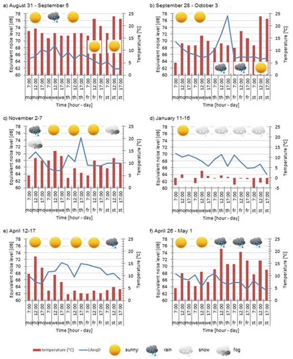
Fig. 8. Changes in the equivalent sound level and air temperature in individual measurement cycles at both sites

Fig. 9. Correlation matrix of the equivalent noise level and day of the week and the measured parameters related to the number of vehicles and weather conditions

In the next part of the analysis, machine learning methods were used to determine the impact of selected factors on the equivalent noise level. The highest values of the determination coefficient were obtained using the support vector method (Fig. 10), for which a satisfactory fit of the forecast data to the observational data was obtained. The values of the Shapley index showed that air temperature had the greatest impact on the fit of the forecast data. The values of this indicator were also influenced by the day of the week, working or not working, and from which measuring site the noise intensity data came from.

In the case of the neural network, the main factors that influenced the results of the noise intensity measurements were temperature, snowfall, and season. According to the ridge regression method, the most important factors that influenced the noise level were temperature, day of the week (working or not), and information about snowfall. In turn, in the nearest-neighbor method, the most valuable information for forecasts was information about the vegetation period, the location of the measurement site, and information about the type of measurement day, working or non-working.

4.5. Discussion of research results

Research carried out showed that in Michałowice, on the DK7 road, the equivalent noise level exceeded the permitted value on weekdays and Saturdays, which was 61 dB for the time of day. Higher values of the equivalent noise level on weekdays, exceeding the permissible values and thus higher than the recorded level on Saturdays, may indicate that the cause is usually higher traffic intensity, which is confirmed, among others, by the studies of Hegewald [23] and Abdur-Rouf and Shaaban [1].

Fig. 10. Comparison of prediction results for
the test and training set using the support vector method

In countries of the European Union, the so-called "noise policy" resulting from Directive 2002/49/EC of the European Parliament and of the Council [12] on the assessment and management of environmental noise. The directive defines objectives and tasks to reduce the harmful impact of excessive noise on the environment. The need to prepare acoustic maps, create "noise combat" programs, and provide residents with access to noise information was highlighted [19]. Acoustic maps are intended to be used for a general diagnosis of noise from various sources in a given area and to forecast changes in the acoustic climate. Acoustic maps are the basis for the preparation of an environmental protection program against noise. The program defines the basic directions and scope of activities necessary to restore acceptable noise levels in the environment.

An acoustic map was prepared for the research site in question, which shows the acoustic climate. An acoustic map allows you to indicate areas and the number of people or residential premises exposed to a specific noise level. The map is developed based on traffic noise measurements and is also the result of modelling acoustic parameters. The research area in question is located in the noise zone allowed for 68 dB, and the average daily traffic intensity for Michałowice ranges from 15 to 29.9 thousand vehicles (Fig. 11). According to the acoustic map, the area directly adjacent to DK7 is in the noise emission range of 70 to 74.9 dB, and the test site itself is in the range of 65 to 69.9 dB. Behind the building line, the emission level is the lowest and is below 59.9 dB. The acoustic map does not indicate any exceedance of the permissible noise level along the analyzed research area.

As part of the RID [43] project implemented in 2016-2018, noise intensity measurements and traffic intensity were carried out, among others, along the national road at the administrative border of the Michałowice and Wilczkowice communes at a distance of approximately 3.0 km from the research (Fig. 12). During the research period, the section of the DK7 road in question had a single-lane 2+1 cross-section (with a slow traffic lane), a 1.0 m wide hard shoulder, and ditches on both sides. The width of individual lanes is approximately 3.5 m, while the width of the entire road is 11 m. The road had a good bituminous surface with numerous patches and local mesh cracks. The transverse unevenness of the road was not maintained throughout the examined section and the roadsides were poorly maintained. There is a vertical concave arch near the buildings.

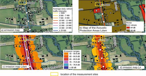
Fig. 11. Acoustic map of the research area in Michałowice
(own study after [55])

The development area included 6 residential buildings located in the Dłubniański Landscape Park with a cantilevered development system (perpendicular to the access road). In terms of height, the buildings are located approximately 2.0 m below the DK7 road and are separated from it by an earth embankment planted with high and low greenery (trees and bushes). To the north of the buildings there are densely planted tall deciduous trees, and in the southern part there are arable fields. The tests were carried out on Friday at 7 sites, the locations of which are shown in Figure 12, in three measurement cycles lasting 15 minutes each and in two repetitions. The results of these tests are presented in Table 2. The measurements were made on Friday in August 2016 during the day in sunny cloudless weather and an average temperature of 25°C.

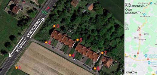
Fig. 12. Location of the measurement sites in RID research (own study after [43, 54])

Comparing the noise level results obtained for the period 2020-2021 with the research conducted as part of the RID project [43] in 2017, it can be concluded that the noise level values were similar (Table 4). Slight differences may result from different locations of measurement sites, time of day, and measurement duration. It can be noted that in the case of research carried out by the National Centre for Research and Development, the distances to the noise source and vehicle speeds were greater and the traffic intensity was lower.

In the case of the RID study [43], the equivalent noise level near DK7 (Fig. 12 – site 1) was the highest, and as they moved away from the road in the development area, they decreased (Fig. 12 – sites 2 to 7). The authors stated that the acoustic climate on the roadside will be unsatisfactory at the beginning of the development system and will improve as we move away from it. The research clearly shows that the existing earth embankment and greenery on the roadside contributed significantly to noise suppression. Measurements of noise spread in the structure of buildings in the area in question showed a reduction in the number of buildings exposed to excessive noise as they moved away from the road.

Tab. 4

Comparison of noise intensity test results (own study after [43])

Parameter		Measurement	RID research [2018] (Michałowice - Wilczkowice border)			Own research (Michałowice)
			Cycle 1	Cycle 2	Cycle 3	Measuring site
			Measuring point
			1,2,3	1,4,5	1,6,7	1	2
Distance from DK7 [m]			25	75	125	11.5	27
Traffic	[l.v. h^-1]^1)	1	744	888	936	884-1402	1000-1508
		2	760	888	868
	[h.v.×h^-1]^2)	1	64	76	88	14-162	98-170
		2	24	108	96
Noise intensity [dB]		1	60.9-71.5	50.4-71.6	50.7-72.8	61.8-71.4	63.0-69.7
		2	61.4-72.2	54.4-72.6	46.5-71.9
^1)l.v. – light vehicles, ^2)l.v. – heavy vehicles

Analyzing the results of research conducted in countries of the European Union, it should be clearly stated that approximately 40% of its inhabitants are exposed to road noise at a level greater than 55 dB [51]. Noise levels in EU countries do not differ from those recorded in other countries. For example, Abdur-Rouf and Shaaban [1] conducted research on road noise levels in the morning, afternoon, and evening hours on weekdays and weekends in Doha, Qatar, and compared them with local limits and the World Health Organization (WHO). As part of the investigation, in addition to measuring sound pressure, they also measured air temperature, humidity, and wind speed. The results obtained showed that, regardless of the day, the average 16-hour noise levels in the selected locations exceeded the allowed values. On weekdays, they ranged from 67.6 dB to 77.5 dB and on weekends from 68.8 dB to 76.9 dB.

Similarly, in other countries, many urban areas are exposed to road noise that exceeds the limit values set by the relevant government authorities of these countries, such as the United States [28, 33], Canada [4, 10], Brazil [9], India [48], Pakistan [35], United Arab Emirates [16, 21]. Most of the time, high noise levels are observed on roads located at major urban intersections, especially in urban areas of developing countries. According to WHO, noise pollution caused by traffic on densely congested roads can be as high as 75-80 dB [51]. However, such noise levels are noticeably higher than the allowed noise thresholds and must be taken into account by governments, urban planners, and policymakers alike.

For many years, countries such as the United Kingdom, the United States, and Australia have recognized road noise as a public health and welfare issue. Therefore, several actions have been taken to reduce road noise levels at the source level by controlling and limiting vehicle use, promoting environmental awareness, introducing sustainable public transport or encouraging cycling. It is also important that these countries have defined guidelines for road design in noise-sensitive areas [8].

Strategies to reduce noise levels by introducing noise-limiting vegetation zones in the city and installing adapted acoustic screens adapted to development where necessary [11, 36, 41, 47]. However, such activities must be related to proper urban planning and land development. This can only be achieved in combination with the implementation of advanced traffic management systems, such as redirecting traffic from highly congested to less congested road networks.

4. CONCLUSION

Based on the analysis of the noise level measurement results, it was found that its equivalent level in individual measurement cycles carried out on the DK7 road in Michałowice from September to May was at a similar level. The location of the research sites and therefore the distance from the DK7 road as a noise source did not show a significant impact on the equivalent noise level. No significant dependencies were found that could significantly influence the research results. Therefore, it can be concluded that loose plantings of coniferous trees and small shrubs do not muffle the noise.

The permissible value of the equivalent noise level for the time of day was found to be exceeded, both for single-family development areas and for service development areas covered by the local development plan at the measurement site. The calculation results indicate that this exceedance occurred for each measurement hour in all measurement cycles at both sites. The measured values of traffic noise were at a high level in relation to the assessment of the subjective feeling of noise annoyance, at the same time, it was an average noise threat.

The distribution of vehicles and the number of passing over time did not change significantly. The exception was on Saturdays when traffic intensity was reduced. Variations in the number of vehicles do not result in a significant reduction in the equivalent noise level. It can be concluded that the influence of the number of cars on the noise level may be distorted by the presence of a speed camera a short distance from the test section. The introduction of a speed camera along the DK7 road in Michałowice and the D-51 road signs informing about its presence resulted in a "calming" of road traffic and adaptation to the permissible speed. The restrictive speed limit of 50 km×h^-1 resulted in the noise level remaining at a similar level during the measurement cycles.

The use of machine learning methods showed that important indirect factors that influence the level of noise generated include air temperature, snowfall, and plant vegetation. Under Polish conditions, where the variability of atmospheric conditions is significant, a more detailed understanding of how these changes affect the equivalent noise level is needed. Research on this phenomenon can contribute to the development of more effective noise management strategies, especially in urban areas where noise is a social and health problem. Implementing countermeasures can contribute to improving the quality of life of residents and creating a more friendly acoustic environment. Significantly lower noise values were obtained during the measurements carried out on the weekend, which shows that the economic nature of traffic dominates in the analyzed road section.

The research shows that with such a significant limitation of car speeds, the permissible value of the equivalent noise level is exceeded. This may result in the need to use noise-absorbing screens. It is proposed to reduce the level of noise by increasing the planting of tree and shrub species native to our climate zone, which will limit the range of noise impact. The use of rigid screens would be more effective, but requires significant financial outlays, which would also reduce the attractiveness of the plots. The construction of the S7 Expressway, whose route is located a considerable distance from Michałowice, is also in favor of limiting the use of rigid screens, which can result in a reduction in vehicle traffic on the analyzed section of the road in the future. Any measures related to the construction of an anti-noise barrier should be preceded by a survey among the residents of Michałowice, as well as the creation of a program co-financing possible additional plantings of trees and shrubs.

It should be noted that during the analysis period, Poland was in the midst of a Covid-19 epidemic, which resulted in the introduction of restrictions that, among other things, recommended limiting movement. The result of these activities was reduced road traffic and, therefore, lower road noise levels.

Acknowledgments

The authors would like to thank MSc Eng. Daniel Wywiał for his help in carrying out the field tests presented in this paper. The authors would like to thank the anonymous reviewers for their efforts towards improving the manuscript.

References

1. Abdur-Rouf K., K. Shaaban. 2022. “Measuring, mapping, and valuating Daytime Traffic Noise Levels at Urban Road Intersections in Doha, Qatar”. Future Transp. 2: 625-643. DOI: 10.3390/futuretransp2030034.

2. Ahmetovic N. 2010. Health and Environment in Europe: Progress Assessment. Technical Report. WHO Regional Office for Europe. ISBN: 978 92 890 4198 0.

3. Andersson E.M, M. Ögren, P. Molnár, D. Segersson, D. Rosengren, L. Stockfelt. 2020. “Road traffic noise, air pollution and cardiovascular events in a Swedish cohort”. Environmental Research 185: 109446. DOI:10.1016/j.envres.2020.109446.

4. Apparicio P., M. Carrier, J. Gelb, A.M. Séguin, S. Kingham. 2016. “Cyclists' exposure to air pollution and road traffic noise in central city neighborhoods of Montreal”. J. Transp. Geogr. 57: 63-69. DOI: 10.1016/j.jtrangeo.2016.09.014.

5. Baranowski J., K. Błażejczyk, P. Milewski. 2014. „Klimat akustyczny w otoczeniu wybranych odcinków dróg w Polsce – wyniki wstępne”. Prace i Studia Geograficzne 56: 17-36. [In Polish: „Acoustic climate in the surrounding of selected sectors of roads in Poland - preliminary results”. Studies in Geography].

6. Berge T., P. Mioduszewski, J. Ejsmont, B. Świeczko-Żurek. 2017. „Reduction of road traffic noise by source measures – present and future strategies”. Noise Control Engineering Journal 65(6): 6. DOI: 10.3397/1/376568.

7. Bortkiewicz A., N. Czaja. 2018. „Pozasłuchowe skutki działania hałasu ze szczególnym uwzględnieniem chorób układu krążenia”. Forum Medycyny Rodzinnej 2(2): 41-49. [In Polish: “Extra-hearing effects of noise, with particular emphasis on cardiovascular diseases”. Family Medicine Forum].

8. Burgess M., J. MacPherson. 2016. “Overview of Australian Road Traffic Noise Policy”. Acoustics Australia 44: 227-234. DOI: 10.1007/s40857-016-0067-2.

9. Calixto A., F.B. Diniz, P.H. Zannin. 2003. “The statistical modeling of road traffic noise in an urban setting”. Cities 20: 23-29. DOI: 10.1016/S0264-2751(02)00093-8.

10. Carrier M., P. Apparicio, A.M. Séguin. 2016. “Road traffic noise in Montreal and environmental equity: What is the situation for the most vulnerable population groups?” J. Transp. Geogr. 51: 1-8. DOI: 10.1016/j.jtrangeo.2015.10.020.

11. Drozd W. 2013. „Ekrany akustyczne jako metoda ograniczenia emisji w infrastrukturze drogowej”. Przegląd budowlany 12: 33-39. [In Polish: “Noise barriers as a method of reducing emissions in road infrastructure”. Builders review].

12. Dyrektywa 2002/49/WE Parlamentu Europejskiego I Rady z dnia 25 czerwca 2002 r. odnosząca się do oceny i zarządzania poziomem hałasu w środowisku. [In Polish: Directive 2002/49/EC of the European Parliament and of the Council of 25 June 2002 relating to the assessment and management of environmental noise.]

13. Dz.U. 2001, nr 62, poz. 627. Ustawa z dnia 27 kwietnia 2001 r. Prawo ochrony środowiska. [In Polish: Journal of Laws 2001, no. 62, item 627. Act of 27 April 2001, Environmental Protection Law.]

14. Dz.U. 2012, poz. 1109. Rozporządzenie Ministra Środowiska z dnia 1 października 2012 r. zmieniające rozporządzenie w sprawie dopuszczalnych poziomów hałasu w środowisku. [In Polish: Journal of Laws 2012, item 1109. Regulation on the Environment Minister of the Environment of October 1, 2012 amending the regulation on allowed noise levels in the environment.]

15. Dz.U. 2014, poz. 112. Obwieszczenie Ministra Środowiska z dnia 15 października 2013 r. w sprawie ogłoszenia jednolitego tekstu rozporządzenia Ministra Środowiska w sprawie dopuszczalnych poziomów hałasu w środowisku. [In Polish: Journal of Laws 2014, item 112. Notice from the Minister of Environment of October 15, 2013 on the publication of the consolidated text of the regulation of Minister of the Environment on allowed noise levels in the environment.]

16. Elmehdi H.M. 2014. “Using mathematical models to predict annoyance from combined noise sources in the city of Dubai”. In: Inter Noise; Citeseer : Melbourne, VIC, Australia.

17. Franklin M., S. Fruin. 2017. “The role of traffic noise on the association between air pollution and children's lung function”. Environmental Research 157: 153-159. DOI: 10.1016/j.envres.2017.05.024.

18. Galli S. 2021. “Feature-engine: A Python package for feature engineering for machine learning”. Journal of Open Source Software 6(65): 3642. DOI: 10.21105/joss.03642.

19. Gardziejczyk W. 2018. Hałaśliwość nawierzchni drogowych. Oficyna Wydawnicza Politechniki Białostockiej, Białystok. ISBN: 978-83-65596-58-1. [In Polish: Noisiness of road surfaces. Publishing House of the Białystok University of Technology, Białystok].

20. GUS 2021. Ochrona środowiska 2021. Główny Urząd Statystyczny, Warszawa. ISSN: 0867-3217. [In Polish: Environment 2021. Statistics Poland, Warsaw].

21. Hamad K., M. Khalil, A. Shanableh. 2017. ”Modeling roadway traffic noise in a hot climate using artificial neural networks”. Transp. Res. Part D Transp. Environ 53: 161-177. DOI: 10.1016/j.trd.2017.04.014

22. Harris C.R., K.J. Millman, S.J. van der Walt, et al. 2020. “Array programming with NumPy”. Nature 585: 357-362. DOI: 10.1038/s41586-020-2649-2.

23. Hegewald J., M. Schubert, M. Lochmann, A. Seidler. 2021. “The burden of disease due to road traffic noise in Hesse, Germany”. Int. J. Environ. Res. Public Health 18: 9337. DOI: 10.3390/ijerph18179337.

24. Hunter J.D. 2007. “Matplotlib: A 2D Graphics Environment”. Computing in Science & Engineering 9(3): 90-95. DOI: 10.1109/MCSE.2007.55.

25. Ibili F., E.K. Adanu, C.A. Adams, S.A. Andam-Akorful, S.S. Turay, S.A. Ajayi. 2021. “Traffic noise models and noise guidelines: A review.” Noise & Vibration Worldwide 53: 1-2. DOI: 10.1177/09574565211052693.

26. Kaleta T. 2022. “Wpływ infrastruktury drogowej i kolejowej na zwierzęta dzikie”. Życie Weterynaryjne 97(2): 81-87. [In Polish: “The effect of roads and railways infrastructure on the wildlife”. Veterinary Life].

27. Koszarny Z., W. Szata. 1987. „Narażenie ludności Warszawy na hałas uliczny. Cz. I i II”. Roczniki Państwowego Zakładu Higieny 38: 1-2. [In Polish: “Traffic noise in the population of Warsaw. Part I and II”. Annals of the Polish National Institute of Hygiene].

28. Lee E.Y., M. Jerrett, Z. Ross, P.F. Coogan, E.Y. Seto. 2014. ”Assessment of traffic-related noise in three cities in the United States”. Environ. Res. 132: 182-189. DOI: 10.1016/j.envres.2014.03.005.

29. Lundberg S.M., G. Erion, H. Chen, A. DeGrave, J.M. Prutkin, B. Nair, R. Katz, J. Himmelfarb, N. Bansal, Su-In Lee. 2020. “From local explanations to global understanding with explainable AI for trees”. Nature Machine Intelligence 2: 56-67. DOI: 10.1038/s42256-019-0138-9.

30. Lundberg Scott M., Su-In Lee. 2017. “A unified approach to interpreting model predictions”. In: Proceedings of 31st Conference on Neural Information Processing Systems (NIPS 2017), Long Beach, CA, USA: 1-10. ISBN: 9781510860964.

31. Malec M., S. Klatka, E. Kruk, M. Ryczek. 2017. „Próba oceny wpływu roślinności na kształtowanie krajobrazu dźwiękowego na przykładzie dwóch parków miejskich Krakowa”. Acta. Sci. Pol., Formatio Circumiectus 16(2): 167-178. DOI: 10.15576/ASP.FC/2017.16.2.167. [In Polish: „An attempt to assess the impact of vegetation on the soundscape on example two urban parks in Krakow”. Acta. Sci. Pol., Formatio Circumiectus].

32. Margaritis E., J. Kang, K. Filipan, D. Botteldooren, 2018. “The influence of vegetation and surrounding traffic noise parameters on the sound environment of urban parks”. Applied Geography 94: 199-212. DOI: 10.1016/j.apgeog.2018.02.017.

33. McAlexander T.P., R.R.M. Gershon, R.L. Neitzel. 2015. “Street-level noise in an urban setting: assessment and contribution to personal impact”. Environ. Health 14: 18. DOI: 10.1186/s12940-015-0006-y.

34. McKinney W. 2010. “Data structures for statistical computing in python”. In: Proceedings of the 9th Python in Science Conference SciPy 2010: 51-56. DOI: 10.25080/Majora-92bf1922-012. June 28 - July 3 2010, Austin, Texas.

35. Mehdi M.R., M. Kim, J.C. Seong, M.H. Arsalan. 2011. “Spatio-temporal patterns of road traffic noise pollution in Karachi, Pakistan”. Environ. Int. 37: 97-104. DOI: 10.1016/j.envint.2010.08.003.

36. Ow L.F., S. Ghosh. 2017. “Urban cities and road traffic noise: Reducing through vegetation”. Appl. Acoust. 120: 15-20. DOI: 10.1016/j.apacoust.2017.01.007.

37. Pedregosa , F., G. Varoquaux, A. Gramfort, V. Michel, B. Thirion, O. Grisel, M. Blondel, P. Prettenhofer, R. Weiss, V. Dubourg, J. Vanderplas, A. Passos, D. Cournapeau, M. Brucher, M. Perrot, E. Duchesnay. 2011. “Scikit -learn: Machine Learning in Python”. Journal of Machine Learning Research 12: 2825-2830.

38. PN-EN 61672-1:2014-03. Elektroakustyka. Mierniki poziomu dźwięku. Część 1: Wymagania. Warszawa: Polski Komitet Normalizacyjny. [In Polish: PN-EN 61672-1:2014-03. Electroacoustics. Sound level meters. Part 1: Requirements. Warsaw: Polish Committee of Standardization].

39. PN-ISO 1996-1:2006. Akustyka. Opis, pomiary i ocena hałasu środowiskowego. Część 1: Wielkości podstawowe i procedury oceny. Warszawa: Polski Komitet Normalizacyjny. [In Polish: PN-ISO 1996-1:2006. Acoustics. Description, measurement and assessment of environmental noise. Part 1: Sizes basic and procedures grades. Warsaw: Polish Committee of Standardization].

40. Poniatowski P. 2022. “The Legal Basis for Protection against Road Traffic Noise: An Outline of the Issue. Part One”. Studies Iuridica Lublinensia 31: 1. DOI: 10.17951/sil.2022.31.1.135-148.

41. Potvin S., P. Apparicio, A.M. Séguin. 2019. “The spatial distribution of noise barriers in Montreal: A barrier to achieving environmental equity”. Transp. Res. Part D Transp. Environ. 72: 83-97. DOI: 10.1016/j.trd.2019.04.011.

42. Puyana-Romero V., J.L. Cueto, R. Gey. 2020. “A 3D GIS tool for the detection of noise hot-spots from major roads”. Transportation Research Part D: Transport and Environment 84: 102376. DOI: 10.1016/j.trd.2020.102376.

43. RID 2018. Rozwój Inicjatyw Drogowych. Projekt RID I/76, Ochrona przed hałasem drogowym. Zadanie 7. Kształtowanie urbanistyczne układów droga w aspekcie ochrony akustycznej ochrony mieszkańców przed hałasem. Available at: http://www.archiwum.gddkia.gov.pl/frontend/web/userfiles/articles/w/wyniki-projektu-rid-ochrona-prze_33468/Zadanie_7.pdf. [In Polish: Development of Road Initiatives. Project RID I/76, Protection against road noise. Task 7. Shaping urban road layouts in terms of acoustic protection and protection of residents against noise].

44. Shannon G., L.M. Angeloni, G. Wittemyer, K.M. Fristrup, K.R. Crooks. 2014. “Road traffic noise modifies behavior of a keystone species”. Animal Behavior 94: 135-141. DOI: 10.1016/j.anbehav.2014.06.004.

45. Szyszlak-Bargłowicz J., T. Słowik, G. Zając. 2012. „Zanieczyszczenia środowiska hałasem komunikacyjnym na terenie Parku Krajobrazowego Pogórza Przemyskiego”. Autobusy: technika, eksploatacja, systemy transportowe 13(10): 144-147. [In Polish: Traffic noise pollution of the Park Krajobrazowy Pogórza Przemyskiego”. Buses: technology, operation, transport systems].

46. Titu A.M., A.A. Boroiu, S. Mihailescu, A.B. Pop, A. Boroiu. 2022. “Assessment of road noise pollution n urban residential areas - a case study in Piteşti, Romania”. Appl. Sci. 12: 4053. DOI: 10.3390/app12084053.

47. Van Renterghem T. 2019. “Towards explaining the positive effect of vegetation on the perception of environmental noise”. Urban Forestry & Urban Greening 40: 133-144. DOI: 10.1016/j.ufug.2018.03.007.

48. Vilas P., N.P. Prashant. 2015. “Measurement and Analysis of Noise at Signalized Intersections”. Journal of Environmental Research And Development 9(03): 662-667.

49. Virtanen P., R. Gommers, T.E. Oliphant, et al. 2020. “SciPy 1.0: fundamental algorithms for scientific computing in Python”. Nature Methods 17: 261-272. DOI: 10.1038/s41592-019-0686-2.

50. Waskom M.L. 2021. “Seaborn: statistical data visualization”. Journal of Open Source Software 6(60): 3021. DOI:10.21105/joss.03021.

51. WHO 2019. “Environmental noise guidelines for the European Region”. World Health Organization. Regional Office for Europe. Copenhagen, Denmark. Available at: http://www.who.int.

52. Wrótny M., J. Bohatkiewicz. 2021. “Traffic Noise and Inhabitant Health – A Comparison of Road and Rail Noise”. Sustainability 13: 7340. DOI: 10.3390/ su13137340.

53. Noise – European Environment Agency. Available at: http://www.eea.europa.eu/en/topics/in-depth/noise.

54. Google maps. Available at: http://www.google.maps.pl.

55. Strategic noise maps. Available at: http://www.gov.pl/web/gddkia/strategiczne-mapy-halasu-2022.

56. Noise – World Health Organization. Available at: http://www.who.int/europe/news-room/fact-sheets/item/noise.

Received 08.10.2024; accepted in revised form 28.01.2025

Scientific Journal of Silesian University of Technology. Series Transport is licensed under a Creative Commons Attribution 4.0 International License

---

[1] Department of Hydraulic Engineering and Geotechnics, University of Agriculture in Kraków, Mickiewicza 24/28, 30-059 Kraków, Poland. Email: andrzej.gruchot@urk.edu.pl. ORCID: https://orcid.org/0000-0002-4752-3357

[2] Department of Hydraulic Engineering and Geotechnics, University of Agriculture in Kraków, Mickiewicza 24/28, 30-059 Kraków, Poland. Email: tymoteusz.zydron@urk.edu.pl. ORCID: https://orcid.org/0000-0003-0413-5386